Parsing portfolio optimization

Our last few posts on risk factor models haven’t discussed how we might use such a model in the portfolio optimization process. Indeed, although we’ve touched on mean-variance optimization, efficient frontiers, and maximum Sharpe ratios in this portfolio series, we haven’t discussed portfolio optimization and its outputs in great detail. If we mean to discuss ways to limit our exposure to certain risks (presumably identified in the risk factor model) while still shooting for a satisfactory (or optimal) risk-adjusted return, we’ll need to investigate optimization in more detail.

Portfolio optimization is a huge topic. Addressing it without delving into all the theory means we’ll gloss over a lot. At the same time, we need to address certain areas to make sure the concepts are at least clear. On this account, the post might be too dry for some or too basic for others. But the prose…well let’s move on.

In our portfolio series, we’ve been using only four assets to capture the major classes of stocks, bonds, commodities, and real estate. Most investment managers use many more assets, but often fewer classes for various reasons: an active management mandate, desire for exposure to higher return assets, in class diversification, or marketing¹. Indeed, academic research shows that the benefits of diversification kick in as the number of assets in a portfolio approaches 30, but flatten out afterward.²

While it is relatively easy to pull the data on 30 stocks, getting a good mix of all the aforementioned asset classes is less so. And, if we wanted to include risk factors with good explanatory power, we’d be spending more time searching and less time writing! Hence, we’ll create ten fake factors and then simulate 30 assets that are explained to varying degrees by those factors.

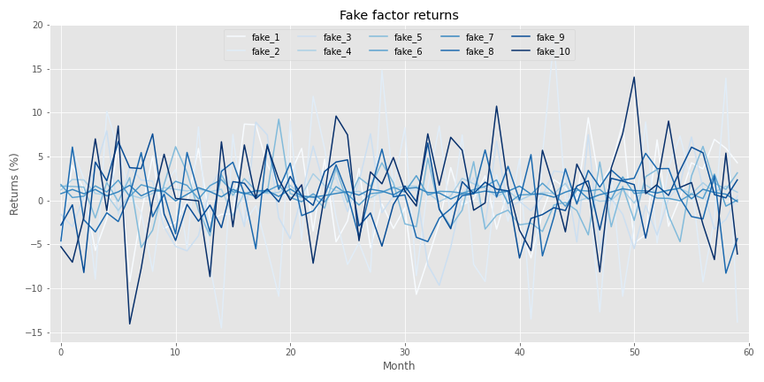
Let’s start by generating fake factors by creating random samples using the same monthly mean and standard deviation as the factors we identified in the last post. Here’s the linguine graph of those factors

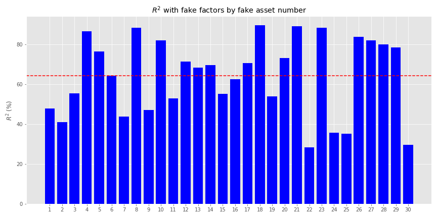
Now we’ll generate returns based on those factors. For those interested, the exact numbers we used to generate the fake returns are in the code below. Briefly, we generated the returns assuming a linear relationship based on the factors including some random noise. The betas (\(\beta\)s) were randomized too. In addition, we added a separate—idiosyncratic, if you will—factor to account for risks one usually doesn’t capture in most risk factor models. We then applied a 90/10 percent weighting to the linear and idiosyncratic generators. Interestingly, this did not mean that the fake factors explained 90% of the asset returns. Rather, they explained a bit more than 60%. as shown in the graph below.

The mean returns have a pretty reasonable distribution, both positive and negative, as we show below. Volatility might a tad low, however.

Now that we’ve got our data generation out of the way, let’s graph our usual portfolio simulation. Here we’ll randomly sample 10,000 different asset weightings as well as randomly exclude up 28 of the assets, equating to 290,000 portfolios. We show the maximum return (blue), maximum Sharpe ratio (red), and minimum volatility portfolio (purple) as well.

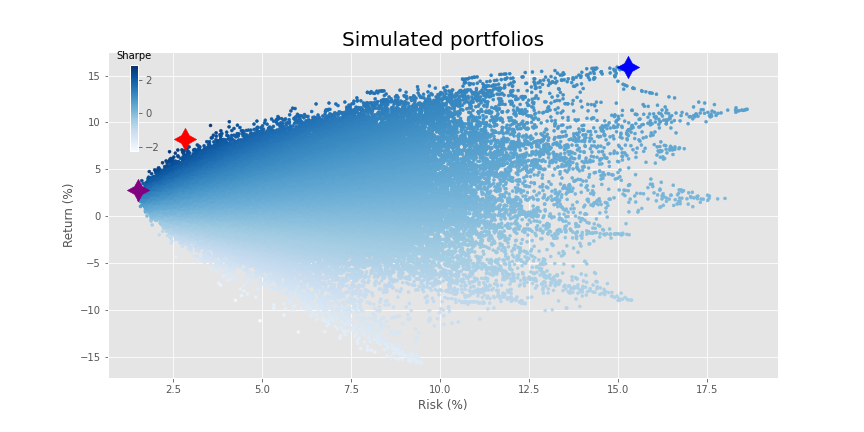
What a fine distribution! Time to run our old favorite—mean-variance optimization (mvo)—so that we can voyage to the efficient frontier.

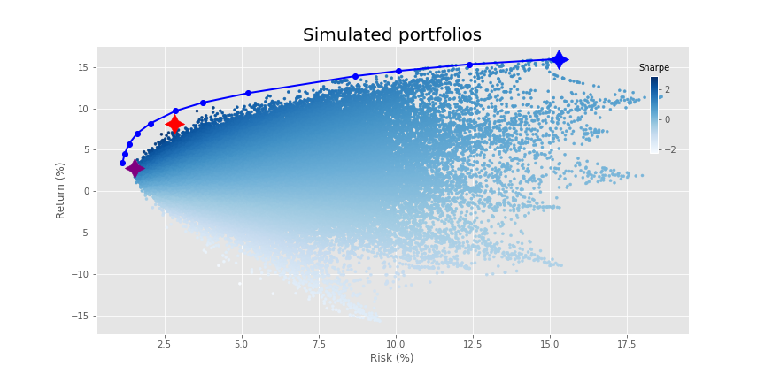
Nice frontier! Interesting that it doesn’t touch most of the portfolios on the lower end of the risk spectrum, but, it still hits the maximum efficient return. This result contrasts with what we saw in our other optimization posts. There, the top end of the distribution aligned almost perfectly with the frontier. We mused, tongue firmly buried in cheek, who needed mvo when you had simulation. What gives?

Time for some combinatorics! Choosing from two up to four out of four assets where order doesn’t matter yields 11 different portfolio combinations: 10 for all the combinations under four assets plus one for the four assets themselves.³ What about thirty assets? 1,073,741,792 plus one.⁴ Add in the infinite space of real numbers between zero and one and that means our sample of 290,000 portfolios didn’t scratch the surface of all possible portfolios and weights. Hence, we were bound to miss some “optimal” combinations that were found by voyaging to the efficient frontier.

This gets at the heart of mvo results. On a large set of assets, many will come, few will be chosen. And even those that are may have a weighting that is small or downright bizarre. Let’s look at an example. Our efficient frontier only calculates 20 optimal portfolios. When we choose the smallest weighting (excluding zero!) for any asset in each portfolio and then graph that weighting we get the following result.

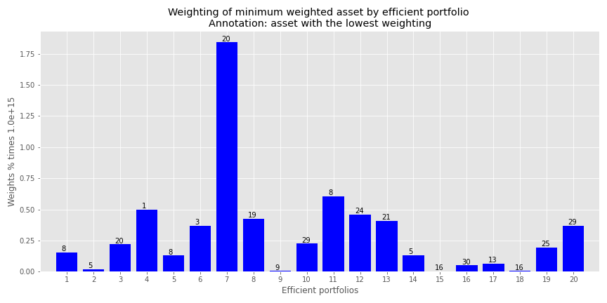
Note the y-axis. The weights are 15 decimal places! Effectively zero, but yielding a portfolio that is unlikely to be implemented unless those 15 decimal place weightings are treated as zero. Where we see those infinitesimally low weightings is the lower risk regions. You only need a small exposure to generate a sufficient return for the least amount of risk. But that exposure is clearly infinitesimal.

This isn’t a criticism of optimization. Indeed, optimization helps because it identifies the highest return to risk, or Sharpe portfolio. Using that you can then achieve a higher return with the same amount of risk as the lower risk portfolios by combining the maximum Sharpe ratio portfolio (the tangency portfolio) with a risk-free asset. Finance wonks know this as the capital market line. But, in this case, since the portfolios represent fake assets (and not even the same number as a traditional market index) we’ve sort of butchered the concept—apologies to the purists.

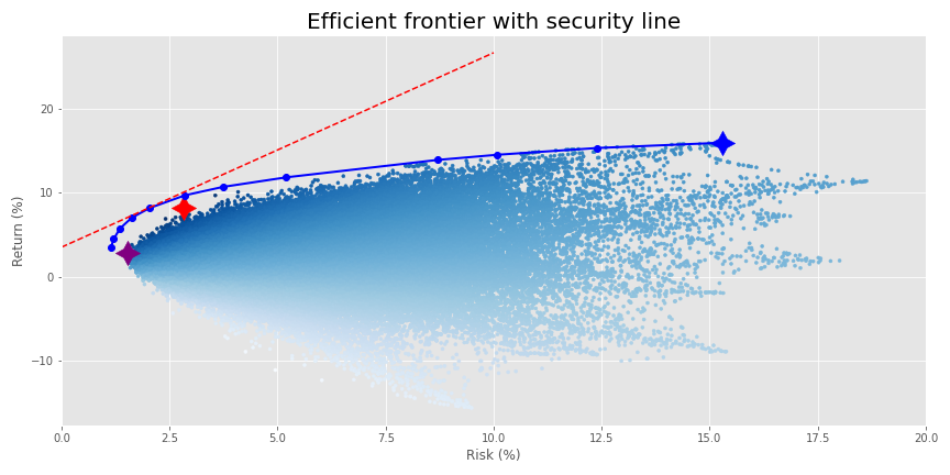
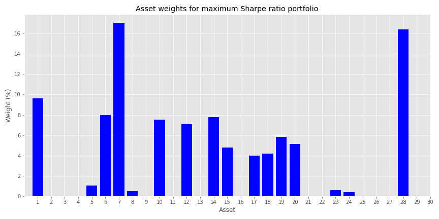
The problem is, even if one were to use only a combination of the maximum Sharpe portfolio and the risk-free asset, it could still leave out a lot of assets. In our example, the maximum Sharpe ratio portfolio on the efficient frontier calculates a weight of less than five basis points (bps) for almost 50% of the assets. We wouldn’t necessarily see this exact percentage on other, real assets for real portfolios, but you get the idea.

Why does this all matter? As we showed in a previous post, the efficient frontier in one period is not necessarily so in the next even for a small group of assets. Hence, it might be better to have some exposure to assets that are considered sub-optimal precisely because the potential for them to contribute to a higher return or lower risk in the next period might be decidedly non-zero. What’s the solution? None perfect, but there are a bunch of workarounds. One would be constrain the weights such that none fall below a pre-determined level. For example, if we limited the minimum weight to 50bps (half a percent), we’d achieve a frontier like the following.

We miss out on some returns on the higher end, but the overall shape looks relatively similar. All that really happens in this case is that about 45% of the assets on the frontier have a 50bps weighting.⁵ For some investors, that might be fine. But for others that still want a bit more of a balanced weighting, they can turn to regularization.

This too is a huge topic in statistics, finance, and machine learning. Hence, we can’t possibly address it in a short post. Suffice it to say that instead of placing a minimum boundary on the weights, regularization penalizes extreme values. This has the effect that large exposures to a couple of assets is reduced, hopefully creating a more balanced weighting scheme. Regularization is “regularly” used in machine learning to prevent overfitting. It is known as a hyperparameter since it’s value is usually provided by the researcher/modeler.

Choosing the right regularization factor, known as hyperparameter tuning, is itself an artful science. Applying grid search and cross-validation can make it a little more scientific. But we won’t do that here. We will show you a couple of regularized frontiers to give one an idea. In later posts, we may perform more detailed tuning.

In the first example of regularization, we simply include the regularization term but don’t adjust the weighting.⁶ This results in the following output.

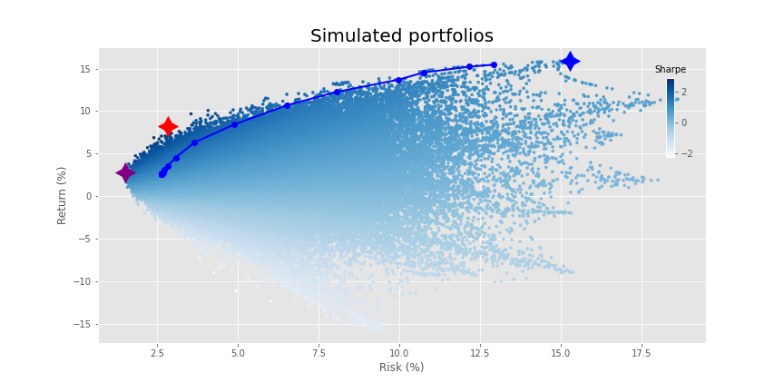
Most of the changes occur at the lower end of the risk spectrum such that the return profile eases a bit. It also clips some of the higher return portfolios. You could offset some of that lost return with the security line scenario we discussed above. But let’s move on. In the next graph, we increase the tuning parameter ten fold.

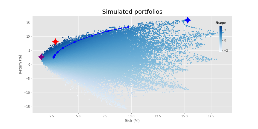
This shortens the line to the maximum return portfolio considerably, but doesn’t seem to change the placement of the lower risk portfolios.

How do the weightings look for the four different optimization outputs? We graph the percentage of assets with weightings under 50bps below.

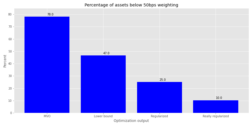
As we can see, constraining the weights removes a good portion of the minimally weighted portfolios, but regularization is even more effective. Unfortunately, this graph doesn’t convey much information about the overall distribution of weights. We provide histograms of the weight outputs for the four different optimization schemes in the next graph. Given that the portfolios contain up to 30 assets, we cut the weighting off at 20%. There are instances above that, but the plot becomes almost unreadable.

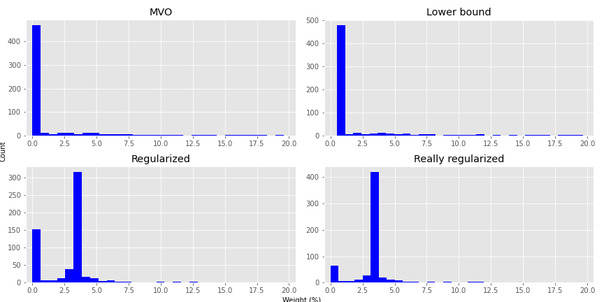
As we hope is clear, most of the weights are pretty close to zero for the MVO portfolios. This distribution isn’t as severe for the Lower Bound constrained portfolios. But the Regularized portfolios see more of the weights around the 3% range; hence, closer to balanced, but with a better risk-adjusted return. Clearly, all the optimized portfolios should enjoy higher Sharpe ratios than an equal weighted portfolio. But it’s interesting that one can get very close to equal weighting using regularization yet still achieve a better risk-adjusted return. This might hold some promise for out-of-sample optimization; we’ll see in later posts.

What are some takeaways? When you start building portfolios with a large number of assets, simulating portfolio weights will likely miss the optimal weighting scheme for a given return or risk profile. Optimization finds those weights. But the output can be impractical or at best ignored in many circumstances. Constraining the weights helps a bit. But regularization tends to work better if the desired outcome is more balance while continuing to offer higher risk-adjusted returns. That presents hope for out-of-sample results. But we’re a ways away from testing that hypothesis. In our next post we’ll begin to explore optimization based on risk factors rather than variance. Until then, here’s the code.

# Built using R 4.0.3 and Python 3.8.3

#[R]
# Load libraries
suppressPackageStartupMessages({
  library(tidyverse)
  library(tidyquant)
  library(reticulate)
  library(png)
  library(grid)
  library(gridExtra)
})

# [Python]
# Load libraries
import warnings
warnings.filterwarnings('ignore')
import numpy as np
import pandas as pd
import statsmodels.api as sm
import matplotlib
import matplotlib.pyplot as plt
import os
os.environ['QT_QPA_PLATFORM_PLUGIN_PATH'] = 'C:/Users/nbwal/Anaconda3/Library/plugins/platforms'
plt.style.use('ggplot')

# Load purpose-built modules and functions
# Code can be found here: https://github.com/nbwosm/optionstocksmachines
from Port_sim_functions import Port_sim as ps
from Portfolio_risk_functions import rsq_func_prem, factor_beta_risk_premium_calc, betas_plot, factor_port_var, port_var_plot

# Load factors
# Prior post (https://www.optionstocksmachines.com/post/2021-01-12-port-22/more-factors-more-variance/) shows how they were downloaded and cleaned.
tf_change = total_factors.copy()
tf_change.loc[:,['PMI', 'ICSA', 'PERMIT', 'BOGMBASE']] = tf_change.loc[:,['PMI', 'ICSA', 'PERMIT', 'BOGMBASE']].pct_change()
tf_change.loc[:,['USSLIND','T10Y2Y', 'CORP']] = tf_change.loc[:,['USSLIND','T10Y2Y', 'CORP']]*.01

# Create time period
fact_gen = tf_change.loc['1990':'2010',[x for x in tf_change.columns.to_list() if x not in ['mkt-rfr', 'rfr']]]

# Generate moments
mu_gen, sig_gen = fact_gen.mean(), fact_gen.std()

# Simulate factors
np.random.seed(123)
fake_factors = pd.DataFrame(np.zeros((60,10)))
for i in range(10):
    fake_factors.iloc[:,i] = np.random.normal(mu_gen[i], sig_gen[i], 60)
    
fake_factors.columns = [f'fake_{i+1}' for i in range(10)]

# Plot fake factors
(fake_factors*100).plot(cmap = 'Blues')
plt.title("Fake factor returns")
plt.xlabel("Month")
plt.ylabel("Returns (%)")
plt.legend(loc = 'upper center', ncol = 5)
plt.show()

# Generate asset returns
np.random.seed(42)
assets = pd.DataFrame(np.zeros((60,30)))
rand_beta = np.array([np.random.normal(0.05,0.3,10) for i in range(30)])
spec_var = np.round(np.random.uniform(0.5,0.9,30),2) #np.repeat(0.9, 30)

for i in range(len(assets.columns)):
    
    assets.iloc[:,i] = spec_var[i]*(np.random.normal(0,0.01/12) + rand_beta[i] @ fake_factors.T + np.random.normal(0.0,0.02,60)) + \
                        (1-spec_var[i])*np.random.normal(0.0, 0.05, 60)
    
assets.columns = [f'asset_{i+1}' for i in range(len(assets.columns))]
assets.head()                  

# Calculate R-squared on assets and graph
rsq = rsq_func_prem(fake_factors, assets, plot=False, print_rsq=False)

plt.figure()
plt.bar([str(x) for x in np.arange(1,31)], rsq, color='blue' )
plt.axhline(np.array(rsq).mean(), color='red', linestyle="--")
plt.title("$R^2$ with fake factors by fake asset number")
plt.ylabel("$R^2$ (%)")
# save_fig_blog('fake_asset_rsq_23')
plt.show()

# Calculate bets
betas, _, error = factor_beta_risk_premium_calc(fake_factors, assets)

# Graph mean return and volatility in Python. The post graphs it in R below
plt.figure()
plt.bar(np.arange(1,31), assets.mean()*1200, color='blue')
plt.axhline(assets.mean().mean()*1200, color='red', linestyle = "--")
plt.title("Mean asset returns")
plt.xlabel("Asset")
plt.ylabel("Return (%)")
plt.show()

asset_sharpe = assets.mean()/assets.std()*np.sqrt(12)*100
plt.figure()
plt.bar(np.arange(1,31), assets.std()*np.sqrt(12)*100, color = 'blue')
plt.title('Asset volatility')
plt.xlabel('Asset')
plt.ylabel('Annualized volatility (%)')
plt.show()

pd.DataFrame(np.c_[assets.mean(), assets.std()], columns = ['return', 'risk']).to_csv('assets_port_23.csv', index=False)

# [R]
# Load asset csv saved from python environment
assets <- read_csv("C:/Users/me/assets_port_23.csv")

assets %>%
  mutate(Portfolio = 1:30,
         Return = Return*1200,
         Risk = Risk*sqrt(12)*100) %>%  
  gather(key,value, -Portfolio)  %>%
  ggplot(aes(factor(Portfolio), value)) +
  labs(y = "Percent",
       x = "Portfolio",
       title = "Fake asset returns and risk") +
  geom_bar(stat="identity", position = 'dodge', fill='blue') +
  scale_x_discrete(breaks = c(1,5,10,15,20,25), expand = c(0.025,0.025))+
  facet_wrap(~key, scales = 'free_y')

# Create portfolio simulations
np.random.seed(42)
port, wts, sharpe  = ps.calc_sim_lv(df = assets, sims = 10000, cols=30)

# Find relevant portfolios and graph simulation
max_sharp = port[np.argmax(sharpe)]
min_vol = port[np.argmin(port[:,1])]
max_ret_eff = port[pd.DataFrame(np.c_[port,sharpe], columns = ['ret', 'risk', 'sharpe']).sort_values(['ret', 'sharpe'], ascending=False).index[0]]

fig = plt.figure()
ax = fig.add_subplot(1,1, 1)
sim = ax.scatter(port[:,1]*np.sqrt(12)*100, port[:,0]*1200, marker='.', c=sharpe, cmap='Blues')
ax.scatter(max_sharp[1]*np.sqrt(12)*100, max_sharp[0]*1200,marker=(4,1,0),color='r',s=500)
ax.scatter(min_vol[1]*np.sqrt(12)*100,min_vol[0]*1200,marker=(4,1,0),color='purple',s=500)
ax.scatter(max_ret_eff[1]*np.sqrt(12)*100,max_ret_eff[0]*1200,marker=(4,1,0),color='blue',s=500)
ax.set_title('Simulated portfolios', fontsize=20)
ax.set_xlabel('Risk (%)')
ax.set_ylabel('Return (%)')

cbaxes = fig.add_axes([0.15, 0.65, 0.01, 0.2])
clb = fig.colorbar(sim, cax = cbaxes)
clb.ax.set_title(label='Sharpe', fontsize=10)
# save_fig_blog('sim_ports_23', tight_layout=False)
plt.show()


# Create efficient factor frontier function
# We found this document helpful in creating the function. If you're curious why we built this using scipy instead of CVXPY or Pyportfolioopt, send us an email and we'll explain.
# https://pyportfolioopt.readthedocs.io/en/latest/index.html

def eff_ret(df_returns, betas=None, factors=None, error=None, gamma=1, optim_out = 'mvo', short = False, l_reg = 0, min_weight = 0):
    
    n = len(df_returns.columns)
    
    def get_data(weights):
        weights = np.array(weights)
        returns = np.sum(df_returns.mean() * weights)
        risk = np.sqrt(np.dot(weights.T, np.dot(df_returns.cov(), weights)))
        sharpe = returns/risk
        return np.array([returns,risk,sharpe])

    def check_sum(weights):
        return np.sum(np.abs(weights)) - 1

    def factor_var_func(weights):
    
        B = np.array(betas)
        F = np.array(factors.cov())
        S = np.diag(np.array(error.var()))

        factor_var = weights.dot(B.dot(F).dot(B.T)).dot(weights.T)
        specific_var = weights.dot(S).dot(weights.T)
         
        return factor_var, specific_var, factor_var/(factor_var + specific_var)
             
    def mvo(weights):
        return -(get_data(weights)[0] - gamma*(get_data(weights)[1]**2 + l_reg*weights.T.dot(weights)))
    
    def factor(weights):
        return -(get_data(weights)[0] - gamma*(factor_var_func(weights)[0] + factor_var_func(weights)[1] + l_reg* weights.T.dot(weights)))
                 
    # Inputs
    init_guess = np.repeat(1/n,n)
    bounds = ((-1 if short else 0, 1),) * n
    
    func_dict = {'mvo': mvo,
                 'factor': factor}
                 
    constraints = {'mvo': ({'type':'eq','fun': check_sum},
                           {'type':'ineq', 'fun': lambda x: x - min_weight}),
                   'factor': ({'type':'eq','fun': check_sum})}
        
    result = minimize(func_dict[optim_out],init_guess,method='SLSQP',bounds=bounds,constraints=constraints[optim_out])
        
    return result.x
    
from scipy.optimize import minimize

# create efficient frontier function
def create_frontier(asset_returns, betas=None, factors=None, error=None, optim_out = 'mvo', short = False, l_reg = 0, min_weight=0):
    
    gammas = np.logspace(-3,3,20)
    gam_wt = []
    for gamma in gammas:
        gam_wt.append(eff_ret(asset_returns, betas, factors, error, gamma, optim_out, short, l_reg, min_weight))

    df_mean = asset_returns.mean()
    df_cov = asset_returns.cov()

    ret_g, risk_g = [], []
    for g in gam_wt:
        ret_g.append(g.T @ df_mean)
        risk_g.append(np.sqrt(g.T @ df_cov @ g))

    return np.array(gam_wt), np.array(ret_g), np.array(risk_g)

def quick_plot(ret_g, risk_g):
    plt.figure()
    plt.plot(risk_g, ret_g, 'bo-')
    plt.show()
    
# Create graph functions to show results
def frontier_plot(portfolios, sharpe_ratios, returns_frontier, risk_frontier, max_sharp, max_ret_eff, min_vol, axes = [0.85, 0.6, 0.01, 0.2],
                 save_fig = False, fig_name=None):
    
    fig = plt.figure()
    ax = fig.add_subplot(1,1, 1)
    ax.scatter(port[:,1]*np.sqrt(12)*100, port[:,0]*1200, marker='.', c=sharpe, cmap='Blues')
    ax.scatter(max_sharp[1]*np.sqrt(12)*100, max_sharp[0]*1200,marker=(4,1,0),color='r',s=500)
    ax.scatter(max_ret_eff[1]*np.sqrt(12)*100,max_ret_eff[0]*1200,marker=(4,1,0),color='blue',s=500)
    ax.scatter(min_vol[1]*np.sqrt(12)*100,min_vol[0]*1200,marker=(4,1,0),color='purple',s=500)
    ax.plot(risk_frontier*np.sqrt(12)*100, returns_frontier*1200, 'bo-', linewidth=2)
    ax.set_title('Simulated portfolios', fontsize=20)
    ax.set_xlabel('Risk (%)')
    ax.set_ylabel('Return (%)')

    cbaxes = fig.add_axes(axes)
    clb = fig.colorbar(sim, cax = cbaxes)
    clb.ax.set_title(label='Sharpe', fontsize=10)
    
    if save_fig:
        save_fig_blog(fig_name, tight_layout=False)

    plt.show()
    
def frontier_wt_plot(frontier_weights, multiplier, nudge, save_fig = False, fig_name=None):
    
    wt_dict = {}
    for num, wts in enumerate(frontier_weights):
        min = 1
        ix = 0
        for idx, wt in enumerate(wts):
            if (wt < min) & (wt > 0):
                min = wt
                ix = idx
        wt_dict[num] = [ix,min] 

    plt.figure()
    vals = [x[1]*multiplier for x in wt_dict.values()]
    labs = [str(x+1) for x in wt_dict.keys()]
    asst = [x[0]+1 for x in wt_dict.values()]

    plt.bar(labs, vals, color = 'blue')

    for i in range(len(wt_dict)):
        plt.annotate(asst[i], xy = (i-0.2, vals[i]+nudge))

    
    plt.xlabel('Efficient portfolios')
    plt.ylabel(f'Weights % times {multiplier/100:.1e}')
    plt.title('Weighting of minimum weighted asset by efficient portfolio \nAnnotation: asset with the lowest weighting')

    if save_fig:
        save_fig_blog(fig_name)

    plt.show()

# Generate first efficient frontier and graph
wt_1, rt_1, rk_1 = create_frontier(assets, 'mvo', l_reg = 0)
max_sharp1 = port[np.argmax(sharpe)]
max_ret_eff1 = port[pd.DataFrame(np.c_[port,sharpe], columns = ['ret', 'risk', 'sharpe']).sort_values(['ret', 'sharpe'], ascending=False).index[0]]
min_vol1 = port[np.argmin(port[:,1])]

frontier_plot(port, sharpe, rt_1, rk_1, max_sharp1, max_ret_eff1, min_vol1, save_fig=False, fig_name = 'eff_front_1_23')

frontier_wt_plot(wt_1, 1e17, 0.01, save_fig = False, fig_name = 'asset_wts_eff_1_23')

# Plot efficient frontier with security line
xs = np.linspace(0,10,20)
slope = (rt_1[np.argmax(sh_1)]*1200)/(rk_1[np.argmax(sh_1)]*np.sqrt(12)*100)-2
ys = xs*slope + 3.5

fig = plt.figure()
ax = fig.add_subplot(1,1, 1)
ax.scatter(port[:,1]*np.sqrt(12)*100, port[:,0]*1200, marker='.', c=sharpe, cmap='Blues')
ax.scatter(max_sharp[1]*np.sqrt(12)*100, max_sharp[0]*1200,marker=(4,1,0),color='r',s=500)
ax.scatter(max_ret_eff[1]*np.sqrt(12)*100,max_ret_eff[0]*1200,marker=(4,1,0),color='blue',s=500)
ax.scatter(min_vol[1]*np.sqrt(12)*100,min_vol[0]*1200,marker=(4,1,0),color='purple',s=500)
# ax.scatter(rk_1[np.argmax(sh_1)]*np.sqrt(12)*100, rt_1[np.argmax(sh_1)]*1200, marker=(4,1,1), color = 'black', s=500)
ax.plot(rk_1*np.sqrt(12)*100, rt_1*1200, 'bo-', linewidth=2)
ax.plot(xs, ys, linestyle="--", color='red')
ax.set_title('Efficient frontier with security line', fontsize=20)
ax.set_xlabel('Risk (%)')
ax.set_ylabel('Return (%)')
ax.set_xlim([0,20])
plt.show()

# Create constrained frontier and graph 
wt_2, rt_2, rk_2 = create_frontier(assets, 'mvo', min_weight = 0.005)
frontier_plot(port, sharpe, rt_2, rk_2, max_sharp1, max_ret_eff1, min_vol1, save_fig=True, fig_name = 'eff_front_2_23')

sh_1 = rt_1/rk_1
sh_w = wt_1[np.argmax(sh_1)]

print(f'{np.mean(sh_w < 0.0005)*100:0.0f}% of the assets are below 5bps in weight')
plt.figure()
plt.bar(np.arange(1,31), sh_w*100, color='blue')
plt.title("Asset weights for maximum Sharpe ratio portfolio")
plt.ylabel("Weight (%)")
plt.xlabel('Asset')
plt.show()

# Create regularized frontier
wt_3, rt_3, rk_3 = create_frontier(assets, 'mvo', l_reg = 1)
frontier_plot(port, sharpe, rt_3, rk_3, max_sharp1, max_ret_eff1, min_vol1, save_fig=True, fig_name='eff_front_3r_23')

# Create really regularize frontier
wt_4, rt_4, rk_4 = create_frontier(assets, 'mvo', l_reg = 10)
frontier_plot(port, sharpe, rt_4, rk_4, max_sharp1, max_ret_eff1, min_vol1, save_fig=True, fig_name = 'eff_front_4r_23')

# Plot weight decline
wt_plot = np.array([np.mean(wt_1 <= 0.005), np.mean(wt_2 <= 0.005), np.mean(wt_3 <= 0.005), np.mean(wt_4 <= 0.005)])
labs = ['MVO', 'Lower bound', 'Regularized', 'Really regularized']
plt.figure()
plt.bar(np.arange(1,5), wt_plot*100, color='blue')
plt.xticks(np.arange(1,5), labs)

for i in range(len(wt_plot)):
    plt.annotate(str(round(wt_plot[i],2)*100), xy = (i+1, wt_plot[i]*100 + 1))
    
plt.title("Percentage of assets below 50bps weighting")
plt.ylabel("Percent")
plt.xlabel("Optimization output")
plt.ylim([0,85])
save_fig_blog('wts_below_50bp_23')

plt.show()

# Plot weight histogram of efficient frontiers
flat_wt_1 = wt_1.flatten()*100
flat_wt_2 = wt_2.flatten()*100
flat_wt_3 = wt_3.flatten()*100
flat_wt_4 = wt_4.flatten()*100

flat_1 = flat_wt_1[flat_wt_1<20]
flat_2 = flat_wt_2[flat_wt_2<20]
flat_3 = flat_wt_3[flat_wt_3<20]
flat_4 = flat_wt_4[flat_wt_4<20]

flat_wts = [flat_1, flat_2, flat_3, flat_4]

fig, axes = plt.subplots(2,2)

for idx, ax in enumerate(fig.axes):
    ax.hist(flat_wts[idx], color='blue', bins=30)
    ax.set_title(labs[idx])
    ax.set_xlim([-0.5,20.5])

plt.subplots_adjust(hspace=0.3)
fig.text(0.005, 0.5, 'Count', ha='center', va='center', rotation=90)
fig.text(0.5, 0.005, 'Weight (%)', ha='center', va='center')
plt.tight_layout()
plt.show()