Risk-constrained optimization

Our last post parsed portfolio optimization outputs and examined some of the nuances around the efficient frontier. We noted that when you start building portfolios with a large number of assets, brute force simulation can miss the optimal weighting scheme for a given return or risk profile. While optimization finds those weights (it should!), the output can lead to infinitesimal contributions from many assets, which is impractical or silly. Placing a minimum on the weights helps a bit. But regularization tends to work better if the desired outcome is more balance while continuing to offer higher risk-adjusted returns.

We introduced some of these optimization concepts and outputs to prepare us to tackle risk-constrained portfolio optimization, which we’ll begin to explore in this post. As we’ve discussed in the last few posts, it would be nice to build a risk factor model that helps to explain a good portion of portfolio variance. Once built, you could limit your exposure to risk factors you wanted to avoid; and dial up the exposure to those you thought might improve returns. If you had identified alpha factors—all the better! You’d increase alpha exposure and try to cancel out the remainder.

Finding the right combination of assets for the desired exposure, all the while maximizing risk-adjusted returns happens to an optimization problem. It also has a computational advantage over mean-variance optimization (MVO). If you’re dealing with lots of investable assets it’s generally faster to run optimizations using risk factor, rather than asset level, covariance matrices. If you’re universe is 500 assets vs. a risk factor model of say 50 features, it will be a lot faster to estimate and optimize a 50 x 50 rather than a 500 x 500 covariance matrix.¹ Of course, if your rebalancing period is measured in months or quarters, then such efficiency may not matter. For shorter time frames, it could become noticeable, however.

We’ll leave the computational complexity discussion for another time; perhaps even another lifetime when the epiphany of R and Python programming strikes us way before we’re able to grow a beard! For this post, we’ll look at some of the outputs of risk factor optimization and try our hand at constraining some of those factors.

Recall, the optimization problem is the following:

maximize: \(\mu^{T}w - \gamma w^{T} \Sigma w\)

subject to \(\mathbf{1}^{T} w = 1\)

Where \(\mu\) = mean return, \(\Sigma\) = covariance matrix, \(w\) = portfolio weights, and \(\gamma\) = risk aversion. In other words, maximize the risk-adjusted returns for a given risk tolerance subject to the asset weights summing to one.

For risk factor optimization, that problem becomes:

maximize: \(\mu^{T}w - \gamma w^{T}(\beta F \beta^{T} + S)w\)

Here \(\beta\) = factor loading matrix, \(F\) = factor covariance matrix, \(S\) = idiosyncratic variance.

Note, our symbolism might not be the most standard, but we hope you get the point. Also, we haven’t always seen the \(\gamma\) term included in risk factor optimization, so don’t focus too closely on that one. What’s the difference between \(\Sigma\) and \(\beta F \beta^{T} + S\)? Quite a lot in intent, not so much in result. The \(\beta\)s are calculated by regressing each asset’s returns against the factors. The factor variance (the \(w^{T}\beta F \beta^{T}w\) part) is the variance explained by the risk factor model, while the specific variance (the \(w^{T}Sw\) part) is what’s not. If the factor and specific variance don’t equal the total variance, then there’s something missing! Remember this because it might be a spoiler for later.

Let’s bring back our portfolio simulations and then run the first optimization. We’ll dispense with the pasta graphs of factor returns. If you miss them, you can click here or here.

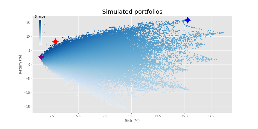
Recall, we created 10 fake factors based on the same risk and return as the macro variables we looked at two posts ago. We then generated 30 asset returns based on random \(\beta\)s, random noise, and a random idiosyncratic factor. We then simulated portfolios consisting of 2 to 30 assets, yielding a beautiful blast of 290,000 portfolios as we show below.

When we ran our mean-variance optimization, our journey to the efficient frontier produced the following.

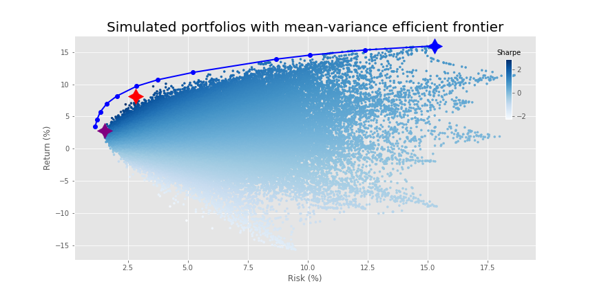
Here, the purple, red, and blue stars are the minimum volatility, maximum Sharpe ratio, and maximum return portfolios based on the simulation. We show them to contrast the results from the simulation with those of the efficient frontier.

Let’s run the optimization using the specific and idiosyncratic variance instead. Do you think it will look different from the graph above?

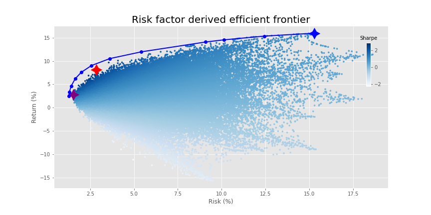
Surprise, surprise. The same graph. Was it that much of a spoiler? We’ll conserve pixels and won’t show the graphs of weight constrained and weight regularized optimizations. They look precisely the same as MVO results. Instead, we’ll examine constraining some of the factors based on risks we want to limit.

Say we don’t want too much risk to housing. We could reduce the \(\beta\) to housing in our portfolio to some number. But what number? First, we would calculate the overall exposure to each factor based on those weights, once we chose a portfolio risk-return profile we liked. Then we’d back in to how much capital was at risk based on that factor. After assessing that number, we’d decide how much we’d like to reduce that capital at risk and constrain accordingly.

When we regress the weighted asset returns for the MVO maximum Sharpe portfolio against the factors, we generate the implied \(\beta\)s, shown in the graph below.

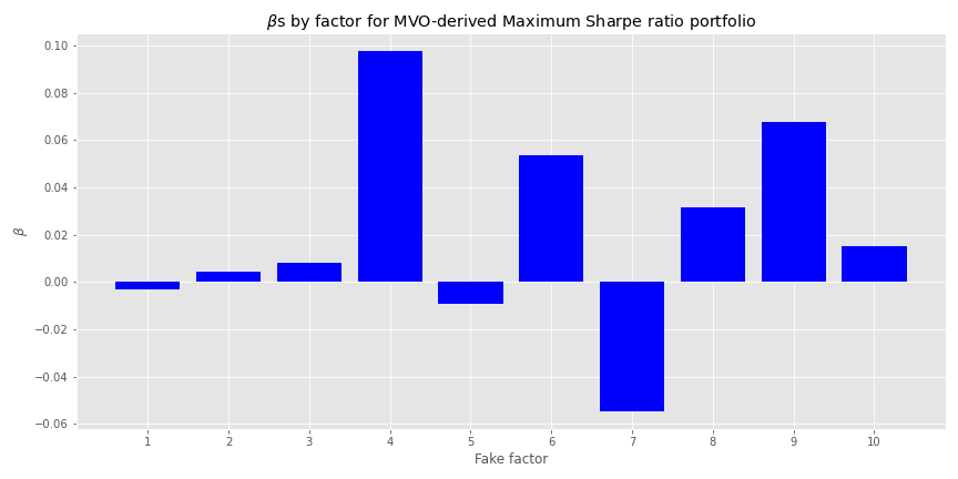
Looks like fake factor 4 exerts a relatively high size effect on the portfolio. If we had a US$100m portfolio, the regression suggests that for every 1% move in fake factor 4, we’d see our portfolio value increase or decrease by US$100k or 10bps. If we don’t want that much risk, we’d constrain that factor to a smaller number or even zero. Let’s say we only want 5bps of exposure. When we run the optimization, constraining just the one factor, we achieve the following frontier. The old maximum Sharpe ratio is in purple, the new one in red. The maximum return portfolio remains in blue.

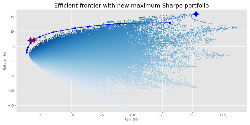
While it appears our return improved, the new maximum Sharpe portfolio actually has a lower Sharpe ratio than the old maximum Sharpe portfolio. In fact, while not easy to see unless you squint, the old Sharpe is not even on the new risk-constrained efficient frontier. Additionally, the frontier doesn’t extend to the maximum return portfolio (in blue) as before.

This somewhat artificial case is clearly for illustration, so there are a few other things we glossed over that would likely alter the results further. For example, the \(\beta\)s we calculated for the maximum Sharpe portfolio were based on returns in which we maintained constant weights on the assets for the calculation period. This implies rebalancing at every period. In practice, most folks aren’t keeping constant weights throughout the period; such rebalancing could be excessive and would also imply increased transaction costs. Setting and forgetting the weights only at the beginning of the period means the weights will deviate (often greatly) from optimal. We’ve touched on this issue in a previous post. But didn’t add those nuances to keep the coding straight forward.

Perhaps we don’t have a strong view on one risk factor, but would prefer to keep our overall exposure to risk factors balanced. We might look at the minimum and maximum factor loadings and pick some mid-point. In the graph below, we plot such loadings across the assets along with the average loading in red.

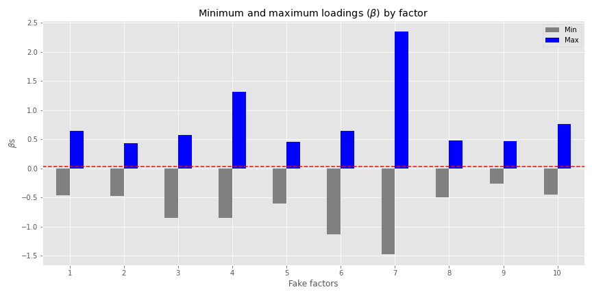
This presents us with a good range of exposures. Note the figures we calculated are based on the 30 assets not the 20 efficient portfolios. The mean \(\beta\) is around 0.033 to 0.038, barely perceptible on the graph were it not for the red line. This is by design, as when we randomized the \(\beta\)s in generating the asset returns (based on the fake factors), we used a mean of 0.05 and standard deviation of 0.30 to try to keep the simulated returns somewhat reasonable.

Whatever the case, in the real word, it’s unlikely that factor size effects would average out close to zero—we’d already be factor neutral without even trying! Of course, just because the average is close to zero, doesn’t mean it would be so easy to calculate asset weights such that all efficient portfolios were close to risk factor neutral.

In any event, if we don’t have a strong view as to which factor exposure we want to reduce or increase, we could simply aim for an overall positive and balanced exposure to take advantage of economic growth (we are looking at macro variables after all!) without too much downside risk. We’ll limit out factor exposure to no less than 5bps. In other words, we want our \(\beta\)s to be no less that 0.05. We graph the resulting frontier below.

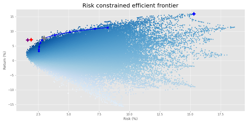
The frontier shrank considerably! The purple and red stars are the Sharpe ratio portfolios from the original MVO frontier and the from the single factor constrained frontier. The gray star is the maximum Sharpe portfolio for the current optimization. Blue is still maximum return.

Let’s confirm that the factor loadings are indeed no less than 5bps. Here we graph the \(\beta\)s of the maximum Sharpe portfolio.

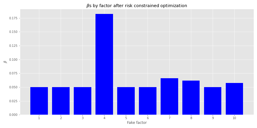
We see that no factor loading is below 0.05. The optimization did exactly what it said on the tin. Of course, the weights for other efficient portfolios won’t be the same, but all the factor loadings will be above 0.05.² Also, fake factor 4 has an even greater size effect. We could re-run the optimization limiting that factor too, but we don’t want to get buried in constraining every factor differently in this post.

A few observations. It shouldn’t be a surprise that the frontier has shrank given how much we were constraining the factor exposure. We were limiting a lot of potential portfolio weights. This could lead to concerns that risk constraints dilute performance. They should. If the fundamental law of finance that more risk equates to more return still holds, then constraining some risks should lead to lower returns. But such a concern might be a paper tiger. Recall the original frontier was based on weights that had effectively zero exposure to half of the assets. Such optimization would be the machine learning equivalent of overfitting. That perfect weighting scheme is unlikely to hold in the future. Additionally, the fact that a good portion of the risk constrained frontier is well within the simulation blast suggests that those weights might not be overly optimized.

Notice that the lower section of the risk constrained frontier is pushed out to the right, implying higher risk. Weren’t we trying to mitigate risk by constraining our exposure to various risk factors? Answering that question fully would take up more space than we have for this post, so we’ll only be able to scratch the surface for now. First, the simple response is that there’s nowhere else to go. The original MVO frontier had already found the minimum. Hence, by reducing the exposure to some factors, we increased others, pushing the minimum factor variance portfolio to the right.

Second, to constrain our exposures, we’re constraining the weights on the explained variance. We didn’t put any constraints on the idiosyncratic variance. Recall, the \(R^{2}\)s for all the assets based on the factors were modestly above 60% on average, but ranged from below 40% to above 80%, as shown in the graph below.

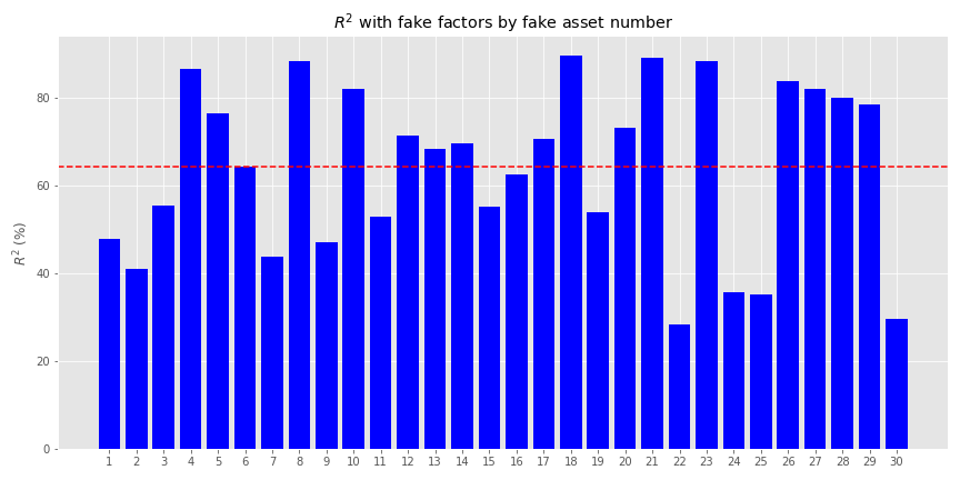
Based on different combinations, the efficient portfolios could have a wide range of \(R^{2}\)s. Optimizing those below 50% would mean we weren’t optimizing for a majority of the variance. Hence, the portfolios could get pushed out along the risk curve.

We’ll want to look at this in more detail in other posts, as well as explore the effect of constraining the idiosyncratic variance.³ For now, we’ll recap.

Risk factor portfolio optimization generates very similar efficient frontiers to mean-variance optimization. However, when one constrains even one of the factors, that frontier tends to shorten. Constrain many of the factors and the efficient portfolios might end up being riskier with lower returns than the original MVO frontier. That might seem contrary to the optimization process, but many MVO portfolios probably overfit the data. So let’s not make perfect (or optimal!) be the enemy of the good.

This post brought up a laundry list of corollary topics to examine. Here are a few.

• Analyzing factor exposures based on initially efficient, but not rebalanced portfolios.
• Setting minimum constraints on factor loadings and/or both minimum and maximum constraints.
• Examining constraining idiosyncratic variance.
• Building risk factor neutral with unconstrained alpha factor portfolios.
• And so much more!

If we’ve missed anything or you want to see one of these topics addressed sooner rather than later, send us a message at the email below. Until next time, here’s the code that makes it all happen.

# Built using R 4.0.3, and Python 3.8.3

# [R]
# Load libraries
suppressPackageStartupMessages({
  library(tidyverse)
  library(tidyquant)
  library(reticulate)
})

# [Python]
# Load libraries
import warnings
warnings.filterwarnings('ignore')
import numpy as np
import pandas as pd
import statsmodels.api as sm
import matplotlib
import matplotlib.pyplot as plt
import os
os.environ['QT_QPA_PLATFORM_PLUGIN_PATH'] = 'C:/Users/user_name/Anaconda3/Library/plugins/platforms'

plt.style.use('ggplot')
plt.rcParams['figure.figsize'] = (12,6)

# Directory to save images
# Most of the graphs are now imported as png. We've explained why in some cases that was necessary due to the way reticulate plays with Python. But we've also found that if we don't use pngs, the images don't get imported into the emails that go to subscribers. 

DIR = "your/image/directory" 

def save_fig_blog(fig_id, tight_layout=True, fig_extension="png", resolution=300):
    path = os.path.join(DIR, fig_id + "." + fig_extension)
    print("Saving figure", fig_id)
    if tight_layout:
        plt.tight_layout()
    plt.savefig(path, format=fig_extension, dip=resolution)

# Import OSM modules and functions
from Port_sim_functions import Port_sim as ps
from Portfolio_risk_functions import rsq_func_prem, factor_beta_risk_premium_calc, betas_plot, factor_port_var, port_var_plot

# Load factors
# Prior post (https://www.optionstocksmachines.com/post/2021-01-12-port-22/more-factors-more-variance/) shows how they were downloaded and cleaned.
tf_change = total_factors.copy()
tf_change.loc[:,['PMI', 'ICSA', 'PERMIT', 'BOGMBASE']] = tf_change.loc[:,['PMI', 'ICSA', 'PERMIT', 'BOGMBASE']].pct_change()
tf_change.loc[:,['USSLIND','T10Y2Y', 'CORP']] = tf_change.loc[:,['USSLIND','T10Y2Y', 'CORP']]*.01

# Create time period
fact_gen = tf_change.loc['1990':'2010',[x for x in tf_change.columns.to_list() if x not in ['mkt-rfr', 'rfr']]]

# Generate moments
mu_gen, sig_gen = fact_gen.mean(), fact_gen.std()

# Simulate factors
np.random.seed(123)
fake_factors = pd.DataFrame(np.zeros((60,10)))
for i in range(10):
    fake_factors.iloc[:,i] = np.random.normal(mu_gen[i], sig_gen[i], 60)
    
fake_factors.columns = [f'fake_{i+1}' for i in range(10)]

# Plot fake factors
(fake_factors*100).plot(cmap = 'Blues')
plt.title("Fake factor returns")
plt.xlabel("Month")
plt.ylabel("Returns (%)")
plt.legend(loc = 'upper center', ncol = 5)
plt.show()

# Generate asset returns
np.random.seed(42)
assets = pd.DataFrame(np.zeros((60,30)))
rand_beta = np.array([np.random.normal(0.05,0.3,10) for i in range(30)])
spec_var = np.round(np.random.uniform(0.5,0.9,30),2) #np.repeat(0.9, 30)

for i in range(len(assets.columns)):
    
    assets.iloc[:,i] = spec_var[i]*(np.random.normal(0,0.01/12) + rand_beta[i] @ fake_factors.T + np.random.normal(0.0,0.02,60)) + \
                        (1-spec_var[i])*np.random.normal(0.0, 0.05, 60)
    
assets.columns = [f'asset_{i+1}' for i in range(len(assets.columns))]

# Calculate betas
betas, _, error = factor_beta_risk_premium_calc(fake_factors, assets)

# Create portfolio simulations
np.random.seed(42)
port, wts, sharpe  = ps.calc_sim_lv(df = assets, sims = 10000, cols=30)

# Find relevant portfolios and graph simulation
max_sharp = port[np.argmax(sharpe)]
min_vol = port[np.argmin(port[:,1])]
max_ret_eff = port[pd.DataFrame(np.c_[port,sharpe], columns = ['ret', 'risk', 'sharpe']).sort_values(['ret', 'sharpe'], ascending=False).index[0]]

fig = plt.figure()
ax = fig.add_subplot(1,1, 1)
sim = ax.scatter(port[:,1]*np.sqrt(12)*100, port[:,0]*1200, marker='.', c=sharpe, cmap='Blues')
ax.scatter(max_sharp[1]*np.sqrt(12)*100, max_sharp[0]*1200,marker=(4,1,0),color='r',s=500)
ax.scatter(min_vol[1]*np.sqrt(12)*100,min_vol[0]*1200,marker=(4,1,0),color='purple',s=500)
ax.scatter(max_ret_eff[1]*np.sqrt(12)*100,max_ret_eff[0]*1200,marker=(4,1,0),color='blue',s=500)
ax.set_title('Simulated portfolios', fontsize=20)
ax.set_xlabel('Risk (%)')
ax.set_ylabel('Return (%)')

cbaxes = fig.add_axes([0.15, 0.65, 0.01, 0.2])
clb = fig.colorbar(sim, cax = cbaxes)
clb.ax.set_title(label='Sharpe', fontsize=10)
# save_fig_blog('sim_ports_23', tight_layout=False)
plt.show()


# Create efficient factor frontier function
# We found this document helpful in creating the function. If you're curious why we built this using scipy instead of CVXPY or Pyportfolioopt, send us an email and we'll explain.
# https://pyportfolioopt.readthedocs.io/en/latest/index.html

def eff_ret(df_returns, betas=None, factors=None, error=None, gamma=1, optim_out = 'mvo', short = False, l_reg = 0, min_weight = 0):
    
    n = len(df_returns.columns)
    
    def get_data(weights):
        weights = np.array(weights)
        returns = np.sum(df_returns.mean() * weights)
        risk = np.sqrt(np.dot(weights.T, np.dot(df_returns.cov(), weights)))
        sharpe = returns/risk
        return np.array([returns,risk,sharpe])

    def check_sum(weights):
        return np.sum(np.abs(weights)) - 1

    def factor_var_func(weights):
    
        B = np.array(betas)
        F = np.array(factors.cov())
        S = np.diag(np.array(error.var()))

        factor_var = weights.dot(B.dot(F).dot(B.T)).dot(weights.T)
        specific_var = weights.dot(S).dot(weights.T)
         
        return factor_var, specific_var, factor_var/(factor_var + specific_var)
             
    def mvo(weights):
        return -(get_data(weights)[0] - gamma*(get_data(weights)[1]**2 + l_reg*weights.T.dot(weights)))
    
    def factor(weights):
        return -(get_data(weights)[0] - gamma*(factor_var_func(weights)[0] + factor_var_func(weights)[1] + l_reg* weights.T.dot(weights)))
                 
    # Inputs
    init_guess = np.repeat(1/n,n)
    bounds = ((-1 if short else 0, 1),) * n
    
    func_dict = {'mvo': mvo,
                 'factor': factor}
                 
    constraints = {'mvo': ({'type':'eq','fun': check_sum},
                           {'type':'ineq', 'fun': lambda x: x - min_weight}),
                   'factor': ({'type':'eq','fun': check_sum})}
        
    result = minimize(func_dict[optim_out],init_guess,method='SLSQP',bounds=bounds,constraints=constraints[optim_out])
        
    return result.x
    
from scipy.optimize import minimize

# create efficient frontier function
def create_frontier(asset_returns, betas=None, factors=None, error=None, optim_out = 'mvo', short = False, l_reg = 0, min_weight=0):
    
    gammas = np.logspace(-3,3,20)
    gam_wt = []
    for gamma in gammas:
        gam_wt.append(eff_ret(asset_returns, betas, factors, error, gamma, optim_out, short, l_reg, min_weight))

    df_mean = asset_returns.mean()
    df_cov = asset_returns.cov()

    ret_g, risk_g = [], []
    for g in gam_wt:
        ret_g.append(g.T @ df_mean)
        risk_g.append(np.sqrt(g.T @ df_cov @ g))

    return np.array(gam_wt), np.array(ret_g), np.array(risk_g)

def quick_plot(ret_g, risk_g):
    plt.figure()
    plt.plot(risk_g, ret_g, 'bo-')
    plt.show()
    
# Create graph functions to show results
def frontier_plot(portfolios, sharpe_ratios, returns_frontier, risk_frontier, max_sharp, max_ret_eff, min_vol, axes = [0.85, 0.6, 0.01, 0.2],
                 save_fig = False, fig_name=None):
    
    fig = plt.figure()
    ax = fig.add_subplot(1,1, 1)
    ax.scatter(port[:,1]*np.sqrt(12)*100, port[:,0]*1200, marker='.', c=sharpe, cmap='Blues')
    ax.scatter(max_sharp[1]*np.sqrt(12)*100, max_sharp[0]*1200,marker=(4,1,0),color='r',s=500)
    ax.scatter(max_ret_eff[1]*np.sqrt(12)*100,max_ret_eff[0]*1200,marker=(4,1,0),color='blue',s=500)
    ax.scatter(min_vol[1]*np.sqrt(12)*100,min_vol[0]*1200,marker=(4,1,0),color='purple',s=500)
    ax.plot(risk_frontier*np.sqrt(12)*100, returns_frontier*1200, 'bo-', linewidth=2)
    ax.set_title('Simulated portfolios', fontsize=20)
    ax.set_xlabel('Risk (%)')
    ax.set_ylabel('Return (%)')

    cbaxes = fig.add_axes(axes)
    clb = fig.colorbar(sim, cax = cbaxes)
    clb.ax.set_title(label='Sharpe', fontsize=10)
    
    if save_fig:
        save_fig_blog(fig_name, tight_layout=False)

    plt.show()
    
def frontier_wt_plot(frontier_weights, multiplier, nudge, save_fig = False, fig_name=None):
    
    wt_dict = {}
    for num, wts in enumerate(frontier_weights):
        min = 1
        ix = 0
        for idx, wt in enumerate(wts):
            if (wt < min) & (wt > 0):
                min = wt
                ix = idx
        wt_dict[num] = [ix,min] 

    plt.figure()
    vals = [x[1]*multiplier for x in wt_dict.values()]
    labs = [str(x+1) for x in wt_dict.keys()]
    asst = [x[0]+1 for x in wt_dict.values()]

    plt.bar(labs, vals, color = 'blue')

    for i in range(len(wt_dict)):
        plt.annotate(asst[i], xy = (i-0.2, vals[i]+nudge))

    
    plt.xlabel('Efficient portfolios')
    plt.ylabel(f'Weights % times {multiplier/100:.1e}')
    plt.title('Weighting of minimum weighted asset by efficient portfolio \nAnnotation: asset with the lowest weighting')

    if save_fig:
        save_fig_blog(fig_name)

    plt.show()

# Generate first efficient frontier and graph
wt_1, rt_1, rk_1 = create_frontier(assets, 'mvo', l_reg = 0)
max_sharp1 = port[np.argmax(sharpe)]
max_ret_eff1 = port[pd.DataFrame(np.c_[port,sharpe], columns = ['ret', 'risk', 'sharpe']).sort_values(['ret', 'sharpe'], ascending=False).index[0]]
min_vol1 = port[np.argmin(port[:,1])]

frontier_plot(port, sharpe, rt_1, rk_1, max_sharp1, max_ret_eff1, min_vol1, save_fig=False, fig_name = 'eff_front_1_23')

# Generate risk factor efficient frontier and graph
wt_f1, rt_f1, rk_f1 = create_frontier(assets, betas, fake_factors, error, optim_out = 'factor', short = False, l_reg = 0)

frontier_plot(port, sharpe, rt_f1, rk_f1, max_sharp1, max_ret_eff1, min_vol1, save_fig=False, fig_name='risk_front_1_24', 
              plot_title='Risk factor derived efficient frontier')


## Create new risk factor constrained optimization function
# We found these links useful:
  # https://nbviewer.jupyter.org/github/dcajasn/Riskfolio-Lib/blob/master/examples/Tutorial%202.ipynb
  # https://riskfolio-lib.readthedocs.io/en/latest/constraints.html
# Note: we're calling it test, becuase is still a work in progress. If it doesn't produce the results you see on the blog, let us know. So many iterations, so little time to check.

def eff_test(df_returns, betas=None, factors=None, error=None, gamma=1, optim_out = 'mvo', 
             short = False, l_reg = 0, min_weight = 0, wt_cons = [[0],[0]]):
    
    n = len(df_returns.columns)
    
    def get_data(weights):
        weights = np.array(weights)
        returns = np.sum(df_returns.mean() * weights)
        risk = np.sqrt(np.dot(weights.T, np.dot(df_returns.cov(), weights)))
        sharpe = returns/risk
        return np.array([returns,risk,sharpe])

    def check_sum(weights):
        return np.sum(np.abs(weights)) - 1

    def factor_var_func(weights):
    
        B = np.array(betas)
        F = np.array(factors.cov())
        S = np.diag(np.array(error.var()))

        factor_var = weights.dot(B.dot(F).dot(B.T)).dot(weights.T)
        specific_var = weights.dot(S).dot(weights.T)
         
        return factor_var, specific_var

    def factor_cons_func(weights):
    
        B = np.array(betas)
        F = np.diag(np.array(factors.var()))
        S = np.diag(np.array(error.var()))

        factor_var = weights.dot(B.dot(F).dot(B.T)).dot(weights.T)
        specific_var = weights.dot(S).dot(weights.T)
         
        return factor_var, specific_var

    def mvo(weights):
        return -(get_data(weights)[0] - gamma*(get_data(weights)[1]**2 + l_reg*weights.T.dot(weights)))
    
    def factor(weights):
        return -(get_data(weights)[0] - gamma*(factor_var_func(weights)[0] + factor_var_func(weights)[1] + l_reg* weights.T.dot(weights)))
    
    def factor_cons(weights):
        return -(get_data(weights)[0] - gamma*(factor_cons_func(weights)[0] + factor_cons_func(weights)[1] + l_reg* weights.T.dot(weights)))
    
    def factor_load(weights):
        B = np.array(betas)
        return weights.dot(B)
    
                 
    # Inputs
    init_guess = np.repeat(1/n,n)
    bounds = ((-1 if short else 0, 1),) * n
    
    func_dict = {'mvo': mvo,
                 'factor': factor,
                 'factor_cons_eq': factor,
                 'factor_cons_ineq': factor}
                 
    constraints = {'mvo': ({'type':'eq','fun': check_sum},
                           {'type':'ineq', 'fun': lambda x: x - min_weight}),
                   'factor': ({'type':'eq','fun': check_sum},
                              {'type':'ineq', 'fun': lambda x: x - min_weight}),
                   'factor_cons_eq': ({'type':'eq','fun': check_sum},
                              {'type':'eq', 'fun': lambda x: factor_load(x)[wt_cons[0]] -                                         wt_cons[1]}),
                    'factor_cons_ineq': ({'type':'eq','fun': check_sum},
                              {'type':'ineq', 'fun': lambda x: factor_load(x)[wt_cons[0]]  -                                      wt_cons[1]})}}
        
    result = minimize(func_dict[optim_out],init_guess,method='SLSQP',bounds=bounds,constraints=constraints[optim_out])
        
    return result.x
    
## Adjust frontier function
def front_test(asset_returns, betas=None, factors=None, error=None, optim_out = 'mvo', short = False, l_reg = 0, min_weight=0, wt_cons = [[0],[0]]):
    
    gammas = np.logspace(-3,3,20)
    gam_wt = []
    for gamma in gammas:
        gam_wt.append(eff_test(asset_returns, betas, factors, error, gamma, optim_out, short, l_reg, min_weight, wt_cons))

    df_mean = asset_returns.mean()
    df_cov = asset_returns.cov()

    ret_g, risk_g = [], []
    for g in gam_wt:
        ret_g.append(g.T @ df_mean)
        risk_g.append(np.sqrt(g.T @ df_cov @ g))

    return np.array(gam_wt), np.array(ret_g), np.array(risk_g)
    
    
## Calculate and graph factor loadings
    
pd.DataFrame(zip(betas.min(), betas.max()), columns = ['Min', 'Max']).plot(kind='bar', color=['grey', 'blue'],figsize=(12,6))
plt.xticks(np.arange(10), labels = [str(x+1) for x in np.arange(10)], rotation=0)
plt.axhline(betas.mean().mean(), color='red', linestyle='--')
plt.xlabel("Fake factors")
plt.ylabel(r"$\beta$s")
plt.title(r'Minimum and maximum loadings ($\beta$) by factor')
save_fig_blog('factor_loadings_24')
plt.show()

## Calculate and graph factor loadings for original MVO max Sharpe portfolio
idx = np.argmax(rt_1/rk_1)

X1 = sm.add_constant(fake_factors.values)
y = assets @ wt_1[idx]
results = sm.OLS(y, X1).fit()
coefs = results.params

plt.figure()
plt.bar(np.arange(1,11), coefs[1:], color="blue")
plt.xticks(np.arange(1,11), [str(x) for x in np.arange(1,11)])
plt.xlabel("Fake factor")
plt.ylabel(r'$\beta$')
plt.title(r'$\beta$s by factor for MVO-derived Maximum Sharpe ratio portfolio')
save_fig_blog('sharpe_betas_24')
plt.show()

## Create constraints on factor 4 and run risk constrained optimization
wt_cons2 = [[3], [0.05]]
wt_t1, rt_t1, rk_t1 = front_test(assets, betas, fake_factors, error, optim_out = 'factor_cons_eq', wt_cons = wt_cons2)


idx1 = np.argmax(rt_1/rk_1)
old_sharpe = np.array([rt_1[idx1], rk_1[idx1]])

idx2 = np.argmax(rt_t1/rk_t1)
new_sharpe = np.array([rt_t1[idx2], rk_t1[idx2]])

fig = plt.figure()
ax = fig.add_subplot(1,1, 1)
ax.scatter(port[:,1]*np.sqrt(12)*100, port[:,0]*1200, marker='.', c=sharpe, cmap='Blues')
ax.scatter(new_sharpe[1]*np.sqrt(12)*100, new_sharpe[0]*1200,marker=(4,1,0),color='r',s=500)
ax.scatter(old_sharpe[1]*np.sqrt(12)*100,old_sharpe[0]*1200,marker=(4,1,0),color='purple',s=500)
ax.scatter(max_ret_eff1[1]*np.sqrt(12)*100,max_ret_eff1[0]*1200,marker=(4,1,0),color='blue',s=500)
ax.plot(rk_t1*np.sqrt(12)*100, rt_t1*1200, 'bo-', linewidth=2)

ax.set_xlabel('Risk (%)')
ax.set_ylabel('Return (%)')

ax.set_title('Efficient frontier with new maximum Sharpe portfolio', fontsize=20)

save_fig_blog('new_sharpe_24', tight_layout=True)

plt.show()

## Create large constraint and run optimization
wt_cons1 = [[np.arange(10)], np.repeat(0.05, 10)]

wt_t, rt_t, rk_t = front_test(assets, betas, fake_factors, error, optim_out = 'factor_cons_ineq', wt_cons = wt_cons1)

idx1 = np.argmax(rt_1/rk_1)
old_sharpe = np.array([rt_1[idx1], rk_1[idx1]])

idx2 = np.argmax(rt_t1/rk_t1)
new_sharpe = np.array([rt_t1[idx2], rk_t1[idx2]])

idx3 = np.argmax(rt_t/rk_t)
cons_sharpe = np.array([rt_t[idx3], rk_t[idx3]])

fig = plt.figure()
ax = fig.add_subplot(1,1, 1)
ax.scatter(port[:,1]*np.sqrt(12)*100, port[:,0]*1200, marker='.', c=sharpe, cmap='Blues')
ax.scatter(new_sharpe[1]*np.sqrt(12)*100, new_sharpe[0]*1200,marker=(4,1,0),color='r',s=200)
ax.scatter(old_sharpe[1]*np.sqrt(12)*100,old_sharpe[0]*1200,marker=(4,1,0),color='purple',s=200)

ax.scatter(max_ret_eff1[1]*np.sqrt(12)*100,max_ret_eff1[0]*1200,marker=(4,1,0),color='blue',s=200)
ax.plot(rk_t*np.sqrt(12)*100, rt_t*1200, 'bo-', linewidth=2)
ax.scatter(cons_sharpe[1]*np.sqrt(12)*100,cons_sharpe[0]*1200,marker=(4,1,0),color='grey',s=400, zorder=4)

ax.set_xlabel('Risk (%)')
ax.set_ylabel('Return (%)')

ax.set_title('Risk constrained efficient frontier', fontsize=20)

save_fig_blog('risk_cons_front_24', tight_layout=True)

plt.show()

## Calculate and graph betas for risk constrained optimization
X1 = sm.add_constant(fake_factors.values)
y = assets @ wt_t[14]
results = sm.OLS(y, X1).fit()
coefs = results.params

plt.figure()
plt.bar(np.arange(1,11), coefs[1:], color="blue")
plt.xticks(np.arange(1,11), [str(x) for x in np.arange(1,11)])
plt.xlabel("Fake factor")
plt.ylabel(r'$\beta$')
plt.title(r'$\beta$s by factor after risk constrained optimization')
save_fig_blog('risk_cons_beta_24')

plt.show()

## R-squareds for fake factors on all assets

plt.figure()
plt.bar([str(x) for x in np.arange(1,31)], rsq, color='blue' )
plt.axhline(np.array(rsq).mean(), color='red', linestyle="--")
plt.title("$R^2$ with fake factors by fake asset number")
plt.ylabel("$R^2$ (%)")
# save_fig_blog('fake_asset_rsq_23')
plt.xlim([-1, len(rsq)-0.025])
plt.show()