Day 1: Benchmarks

Yesterday we set out our plan to backtest a strategy using the SPY ETF, which tracks the S&P 500. Before we commence, we obviously need to establish a baseline. What metrics will we use to assess the strategy? How will we define success? What benchmarks will we use? Typically, for a single asset strategy the comparison is buy-and-hold performance. That is, if you’re using Fibonacci retracements with Bollinger Band breakouts filtered by Chaikin Volatility to generate buy and sell signals, you’ll usually compare the performance of that strategy to one in which you bought the underlying on the first day of the test and held it until the end.

While that is a fair way of starting, it has some unrealistic assumptions – most notably that one would have bought precisely on the day the backtest started. As the highly respected Marcos Lopéz de Prado cautions in Advances in Financial Machine Learning, “a standard backtest is a historical simulation, which can be easily overfit. History is just the random path that was realized, and it could have been entirely different.” We think this has a corollary – namely, your choice of starting point for the benchmark is also a random path. Whatever the case, we need to start somewhere, so we’ll stick with buy-and-hold as a baseline, but include other benchmarks too. For example, most folks have some exposure to bonds. So it might be worthwhile to include a portfolio that has such exposure too. For this we’ll use the IEF ETF, which tracks 7-10 year US Treasury Notes. What equity/bond split will we use? Although the news of 60-40 being dead has been greatly exaggerated, we plan to use that or maybe a 50-50 portfolio. In other words, we’ll be comparing the strategy against a portfolio of 60%/40% or 50%/50% SPY and IEF.

Next we choose our period. Longer is usually better for backtests, which falls under the rule-of-thumb that more data is generally better. Of course, it’s really more better data that’s better. But that discussion and movies about conflicted jazz musicians will have to wait for another time. The main point is we need enough data to ensure we’re capturing more than one regime and not too much that the bulk of it is irrelevant to investment decisions we plan to make today, tomorrow, and tomorrow. With that in mind we’ll opt for ad hoc over rigor and use the period starting in 2019.¹

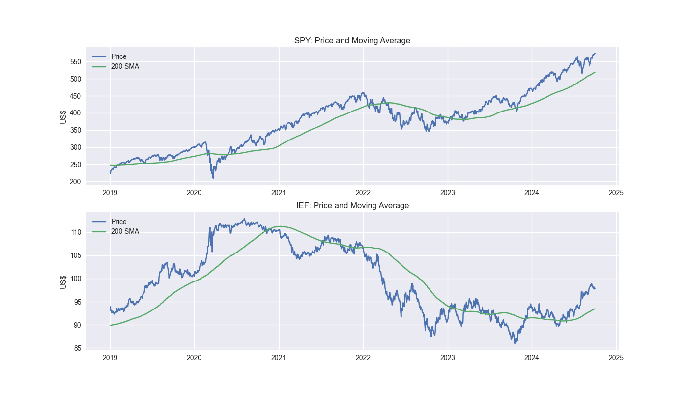
Let’s ground ourselves by looking at the five-year charts of our two ETFs along with the 200-day moving average.

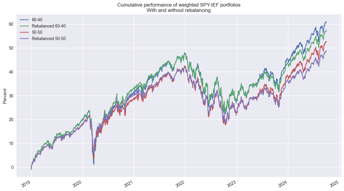
Now we’ll look at the cumulative performance of different weighting schemes – 60/40 vs. 50/50 SPY/IEF – with and without quarterly rebalancing. Interestingly, the non-rebalanced 60/40 portfolio outperforms the 50-50 rebalanced portfolio by more than 12 percentage points over the period. The Sharpe Ratios are about the same. We’ll go into detail on all these metrics tomorrow. Code below.

# Load packages
import os
import pandas as pd
import numpy as np
from datetime import datetime, timedelta
import statsmodels.api as sm
import matplotlib.pyplot as plt
from matplotlib.ticker import FuncFormatter
from utils_intraday import *

plt.style.use('seaborn-v0_8')
plt.rcParams['figure.figsize'] = (14,8)


# Load Data
data = yf.download(['SPY', 'IEF'], start='2000-01-01', end='2024-10-01')
data.head()

# Clean up
df = data.loc["2003-01-01":, 'Adj Close']
df.columns.name = None
tickers = ['ief', 'spy']
df.index.name = 'date'
df.columns = tickers

# Add features
df[['ief_chg', 'spy_chg']] = df[['ief','spy']].apply(lambda x: np.log(x/x.shift(1)))
df[['ief_200sma', 'spy_200sma']] = df[['ief','spy']].rolling(200).mean()

for ticker in tickers:
    df[f"{ticker}_signal"] = np.where(df[ticker] > df[f"{ticker}_200sma"], 1 , 0)
    df[f"{ticker}_strat"] = df[f"{ticker}_chg"]*df[f"{ticker}_signal"].shift(1)

# Plot 200SMA
fig, (ax1, ax2) = plt.subplots(2,1)

top = df.loc['2019-01-01':, ['spy', 'spy_200sma']]
bottom = df.loc['2019-01-01':, ['ief', 'ief_200sma']]

ax1.plot(top.index, top.values)
ax1.set_xlabel("")
ax1.set_ylabel("US$")
ax1.legend(['Price', '200 SMA'], loc="upper left")
ax1.set_title("SPY: Price and Moving Average")

ax2.plot(bottom.index, bottom.values)
ax2.set_xlabel("")
ax2.set_ylabel("US$")
ax2.legend(['Price', '200 SMA'], loc="upper left")
ax2.set_title("IEF: Price and Moving Average")

plt.show()

# Create dataframe for benchmark portfolios
returns = df[['ief_chg', 'spy_chg']].copy()
returns = returns.loc['2019-01-01':]

# Define function to calculate portfolio performance with/out rebalancing
def calculate_portfolio_performance(weights: list, returns: pd.DataFrame, rebalance=False, frequency='month') -> pd.Series:
    # Initialize the portfolio value to 0.0
    portfolio_value = 0.0
    portfolio_values = []

    # Initialize the current weights
    current_weights = np.array(weights)

    # Create a dictionary to map frequency to the appropriate offset property
    frequency_map = {
        'week': 'week',
        'month': 'month',
        'quarter': 'quarter'
    }

    if rebalance:
        # Iterate over each row in the returns DataFrame
        for date, daily_returns in returns.iterrows():
            # Apply the current weights to the daily returns
            portfolio_value = np.dot(current_weights, daily_returns)
            portfolio_values.append(portfolio_value)

            # Rebalance at the selected frequency (week, month, quarter)
            offset = pd.DateOffset(days=1)
            next_date = date + offset

            # Dynamically get the attribute based on frequency
            current_period = getattr(date, frequency_map[frequency])
            next_period = getattr(next_date, frequency_map[frequency])

            if current_period != next_period:
                current_weights = np.array(weights)
            else:
                # Update weights based on the previous day's returns
                current_weights = current_weights * (1 + daily_returns)
                current_weights /= np.sum(current_weights)
    else:
        # No rebalancing, just apply the initial weights
        for date, daily_returns in returns.iterrows():
            portfolio_value = np.dot(current_weights, daily_returns)
            portfolio_values.append(portfolio_value)

            # Update weights based on the previous day's returns
            current_weights = current_weights * (1 + daily_returns)
            current_weights /= np.sum(current_weights)

    daily_returns = pd.Series(portfolio_values, index=returns.index)

    return daily_returns

# Create portfolios
# 60/40
weights = [0.4,0.6]
port_60_40_no_rebal = calculate_portfolio_performance(weights, returns)
port_60_40_rebal = calculate_portfolio_performance(weights, returns, rebalance=True, frequency='quarter')

# 50/50
weights = [.5, .5]
port_50_50_no_rebal = calculate_portfolio_performance(weights, returns, rebalance=False, frequency='quarter')
port_50_50_rebal = calculate_portfolio_performance(weights, returns, rebalance=True, frequency='quarter')

# Plot 60/40 and 50/50
(pd.concat([port_60_40_no_rebal, port_60_40_rebal, port_50_50_no_rebal, port_50_50_rebal], axis=1).cumsum()*100).plot()
plt.legend(['60-40', 'Rebalanced 60-40', '50-50', 'Rebalanced 50-50'])
plt.ylabel('Percent')
plt.xlabel('')
plt.title('Cumulative performance of weighted SPY-IEF portfolios\nWith and without rebalancing')
plt.show()