Day 2: Hello World

On Day 1, we decided on a few benchmarks to use for our backtest. That is, a 60-40 and 50-50 weighting of the SPY and IEF ETFs. What we want to add in now is the Hello World version of trading strategies – the 200-DAY MOVING AVERAGE! Why are we adding this to our analysis? As we pointed out yesterday, the typical benchmark against which to compare a trading strategy is buy-and-hold. But, just as a backtest is random historical occurrence on the strategy side, so is the buy-and-hold. A fairer or more realistic benchmark is another simple (naive?) rules-based strategy. Enter the 200-day moving average, which we’ll abbreviate to 200SMA (simple moving average).

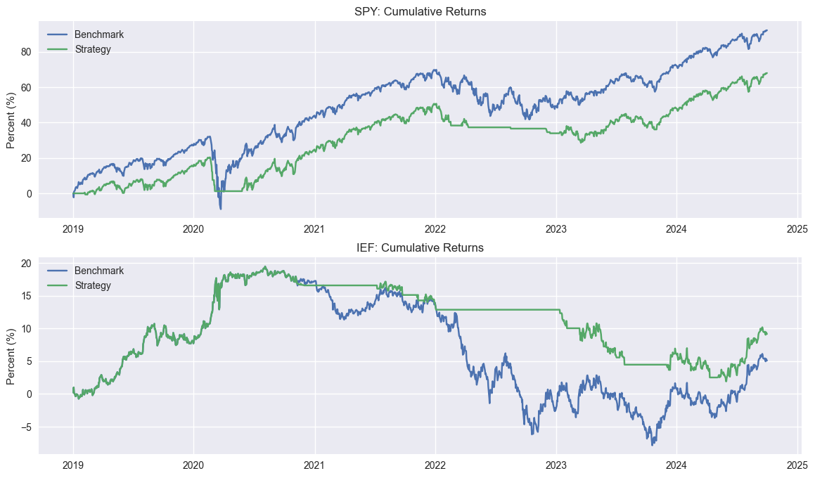
Still not convinced why the 200SMA warrants inclusion? The reality is no one really buys-and-holds – not even Warren Buffett.¹ So we need some way to approximate the fact that a realistic scenario is one where the investor is buying and selling the underlying for a reason other than noise.² The 200SMA has a logical basis for usage, is well-known, and was even used by some academics³ if you can believe it! So let’s look briefly at what a 200SMA strategy would look like when applied to the SPY and IEF. We’ve already shown the two ETFs with the 200SMA in our previous post, so you can have a gander there. Here’s a double plot showing cumulative returns to Buy-and-Hold (Benchmark) and the 200SMA (Strategy).

As one can see, the SPY 200SMA underperforms Buy-and-Hold, while it’s quite the opposite for IEF. Of course, we know the main culprit for such performance on the bond side is the jump in Fed Funds Rate from almost nothing to over 5% in 2022 and 2023.

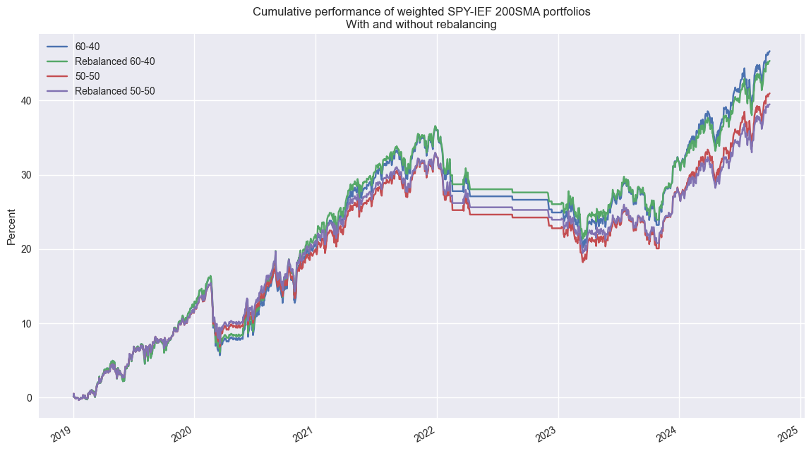
Now let’s look at cumulative return plots of the 60-40 and 50-50 portfolios using the 200SMA strategy. As with the Buy-and-Hold we showed yesterday, the non-rebalanced 60/40 portfolio outperforms the 50-50 rebalanced portfolio and the Sharpe Ratios are about the same.

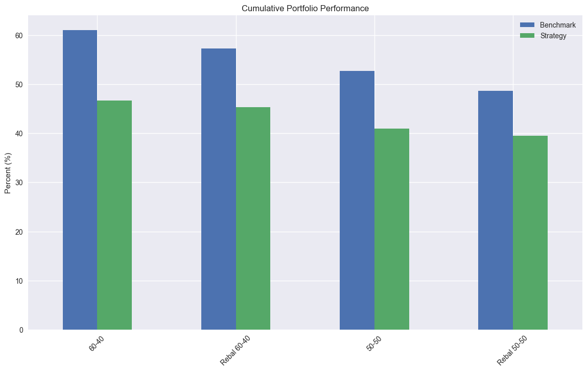
However, when we compare the two strategies and their respective portfolios we some interesting results. The 200SMA portfolios underperform Buy-and-Hold on cumulative performance…

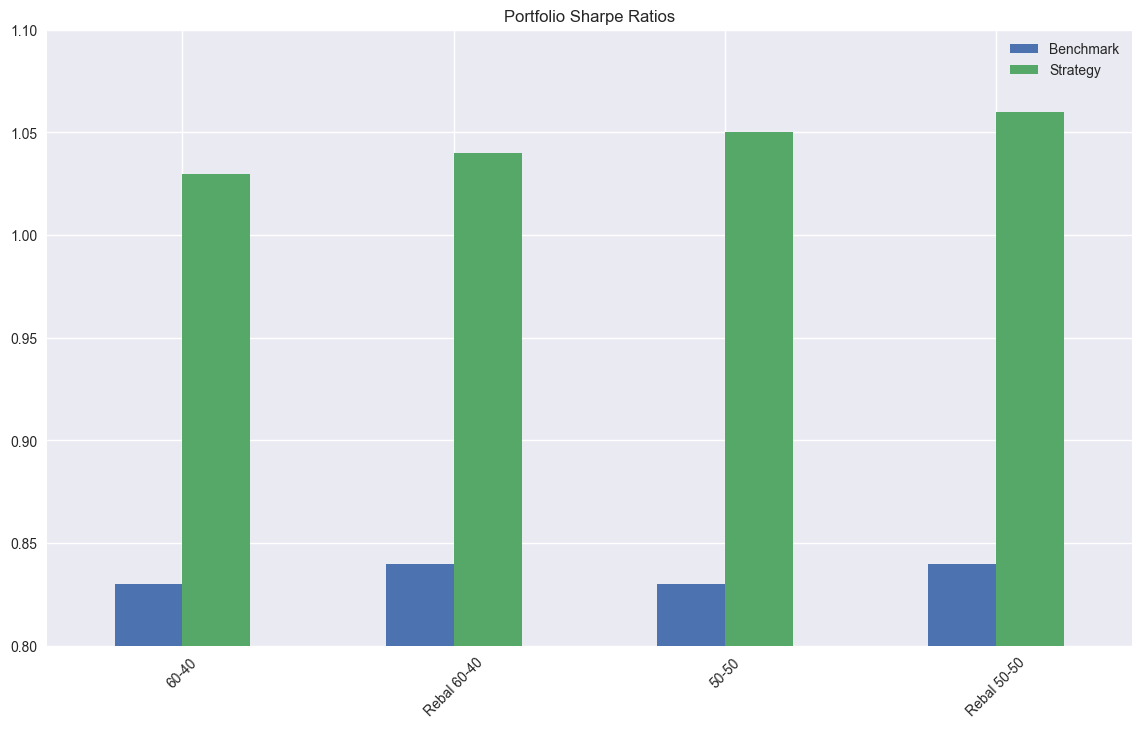
…but outperform on risk-adjusted performance using the Sharpe Ratio.

Tomorrow we’ll look at some the performance metrics we’re thinking of using. Code below.

# Built using Python 3.10.19 and a virtual environment 

# Load packages
import pandas as pd
import numpy as np
from datetime import datetime, timedelta
import statsmodels.api as sm
import matplotlib.pyplot as plt

plt.style.use('seaborn-v0_8')
plt.rcParams['figure.figsize'] = (14,8)


# Load Data
data = yf.download(['SPY', 'IEF'], start='2000-01-01', end='2024-10-01')
data.head()

# Clean up
df = data.loc["2003-01-01":, 'Adj Close']
df.columns.name = None
tickers = ['ief', 'spy']
df.index.name = 'date'
df.columns = tickers

# Add features
df[['ief_chg', 'spy_chg']] = df[['ief','spy']].apply(lambda x: np.log(x/x.shift(1)))
df[['ief_200sma', 'spy_200sma']] = df[['ief','spy']].rolling(200).mean()

for ticker in tickers:
    df[f"{ticker}_signal"] = np.where(df[ticker] > df[f"{ticker}_200sma"], 1 , 0)
    df[f"{ticker}_strat"] = df[f"{ticker}_chg"]*df[f"{ticker}_signal"].shift(1)

# Plot cumulative performance    
fig, (ax1, ax2) = plt.subplots(2,1)

top = df.loc['2019-01-01':, ['spy_chg', 'spy_strat']].cumsum()*100
bottom = df.loc['2019-01-01':, ['ief_chg', 'ief_strat']].cumsum()*100

ax1.plot(top.index, top.values)
ax1.set_xlabel("")
ax1.set_ylabel("Percent (%)")
ax1.legend(['Benchmark', 'Strategy'], loc="upper left")
ax1.set_title("SPY: Cumulative Returns")

ax2.plot(bottom.index, bottom.values)
ax2.set_xlabel("")
ax2.set_ylabel("Percent (%)")
ax2.legend(['Benchmark', 'Strategy'], loc="upper left")
ax2.set_title("IEF: Cumulative Returns")

plt.show()

# Create dataframe for benchmark portfolios
bench_returns = df[['ief_chg', 'spy_chg']].copy()
bench_returns = bench_returns.loc['2019-01-01':]

strat_returns = df[['ief_strat', 'spy_strat']].copy()
strat_returns = strat_returns.loc['2019-01-01':]

# Define function to calculate portfolio performance with/out rebalancing
def calculate_portfolio_performance(weights: list, returns: pd.DataFrame, rebalance=False, frequency='month') -> pd.Series:
    # Initialize the portfolio value to 0.0
    portfolio_value = 0.0
    portfolio_values = []

    # Initialize the current weights
    current_weights = np.array(weights)

    # Create a dictionary to map frequency to the appropriate offset property
    frequency_map = {
        'week': 'week',
        'month': 'month',
        'quarter': 'quarter'
    }

    if rebalance:
        # Iterate over each row in the returns DataFrame
        for date, daily_returns in returns.iterrows():
            # Apply the current weights to the daily returns
            portfolio_value = np.dot(current_weights, daily_returns)
            portfolio_values.append(portfolio_value)

            # Rebalance at the selected frequency (week, month, quarter)
            offset = pd.DateOffset(days=1)
            next_date = date + offset

            # Dynamically get the attribute based on frequency
            current_period = getattr(date, frequency_map[frequency])
            next_period = getattr(next_date, frequency_map[frequency])

            if current_period != next_period:
                current_weights = np.array(weights)
            else:
                # Update weights based on the previous day's returns
                current_weights = current_weights * (1 + daily_returns)
                current_weights /= np.sum(current_weights)
    else:
        # No rebalancing, just apply the initial weights
        for date, daily_returns in returns.iterrows():
            portfolio_value = np.dot(current_weights, daily_returns)
            portfolio_values.append(portfolio_value)

            # Update weights based on the previous day's returns
            current_weights = current_weights * (1 + daily_returns)
            current_weights /= np.sum(current_weights)

    daily_returns = pd.Series(portfolio_values, index=returns.index)

    return daily_returns

# Calculate performance
# 60-40
weights = [0.4,0.6]
bench_60_40_no_rebal = calculate_portfolio_performance(weights, bench_returns)
bench_60_40_rebal = calculate_portfolio_performance(weights, bench_returns, rebalance=True, frequency='quarter')

# 50-50
weights = [.5, .5]
bench_50_50_no_rebal = calculate_portfolio_performance(weights, bench_returns, rebalance=False, frequency='quarter')
bench_50_50_rebal = calculate_portfolio_performance(weights, bench_returns, rebalance=True, frequency='quarter')

# Plot performance
(pd.concat([bench_60_40_no_rebal, bench_60_40_rebal, bench_50_50_no_rebal, bench_50_50_rebal], axis=1).cumsum()*100).plot()
plt.legend(['60-40', 'Rebalanced 60-40', '50-50', 'Rebalanced 50-50'])
plt.ylabel('Percent')
plt.xlabel('')
plt.title('Cumulative performance of weighted SPY-IEF Buy-and-Hold portfolios\nWith and without rebalancing')
plt.show()

# Create portfolio dataframes
bench_peformance = pd.DataFrame((pd.concat([bench_60_40_no_rebal, bench_60_40_rebal, bench_50_50_no_rebal, bench_50_50_rebal], 
                        axis=1).cumsum()*100).iloc[-1].round(2).values,
                        columns=['Benchmark'],
                        index=['60-40', 'Rebal 60-40', '50-50', 'Rebal 50-50'])


bench_sharpes = pd.DataFrame(pd.concat([bench_60_40_no_rebal, bench_60_40_rebal, bench_50_50_no_rebal, bench_50_50_rebal], 
                                 axis=1).apply(lambda x: x.mean()/x.std()*np.sqrt(252)).round(2).values,
                                 columns=['Benchmark'],
                        index=['60-40', 'Rebal 60-40', '50-50', 'Rebal 50-50'])

strat_performance = pd.DataFrame((pd.concat([strat_60_40_no_rebal, strat_60_40_rebal, strat_50_50_no_rebal, strat_50_50_rebal], 
                        axis=1).cumsum()*100).iloc[-1].round(2).values,
                        columns=['Strategy'],
                        index=['60-40', 'Rebal 60-40', '50-50', 'Rebal 50-50'])


strat_sharpes = pd.DataFrame(pd.concat([strat_60_40_no_rebal, strat_60_40_rebal, strat_50_50_no_rebal, strat_50_50_rebal], 
                                 axis=1).apply(lambda x: x.mean()/x.std()*np.sqrt(252)).round(2).values,
                                 columns=['Strategy'],
                        index=['60-40', 'Rebal 60-40', '50-50', 'Rebal 50-50'])

# Plot cumulative portfolio performance
pd.concat([bench_peformance, strat_performance], axis=1).plot(kind='bar', rot=45)
plt.ylabel('Percent (%)')
plt.title('Cumulative Portfolio Performance')
plt.show()

# Plot portfolio Sharpe ratios
pd.concat([bench_sharpes, strat_sharpes], axis=1).plot(kind='bar', rot=45)
plt.ylabel('')
plt.ylim(0.8,1.1)
plt.title('Portfolio Sharpe Ratios')
plt.show()