Day 4: First analysis
We’re four days in and you’re probably wondering when are we actually going to start backtesting?! The answer is that while it is natural to want to rush to the fun part – the hope and elation of generating outsized returns and Sharpe Ratios greater than 2 – the reality is getting the foundation right should serve us well in the future. Or so that’s what we always hear from those longer in the tooth. We admit that we’re just as prone to the allure of backtest first, figure out the benchmarks later as the next big swinging person. But like Epictetus we must strive for (if not achieve) πειθαρχία or disciplina for the Roman Stoics.1
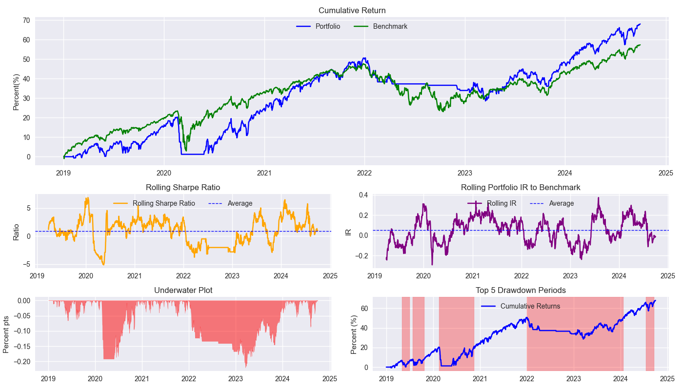
Recall, we opted for the following metrics to judge our strategy: cumulative return, the Sharpe Ratio, and max drawdown. We put all these into a handy tear sheet, which we show below. In this case, the strategy is the 200-day simple moving average (200SMA) vs the benchmark 60%/40% SPY/IEF allocation rebalanced every quarter.

A few observations. The strategy essentially tracks the benchmark throughout much of the backtest period. While it does keep one out of the market in 2022 (as shown by the horizontal line), it pretty much pooped the proverbial bed in 2020. The strategy was underperforming and sold right at the bottom. Of course, that was the beginning of Covid-19, so maybe one can forgive this one. Whatever the case, the rolling Sharpe Ratio looks volatile, but isn’t that bad at an average of close to one. The rolling information ratio, which measures the difference between portfolio and benchmark returns and divides that by the standard deviation of that difference, is paltry – about 0.05 on average. The underwater plot shows us various drawdowns from recent peaks. Interestingly, 2023 was the worst, followed closely by 2020. This is instructional because the psychological impact of being out of the market for a good portion of the year only to return and lose money right away is a real challenge. Finally, the drawdown period graph shows the duration of sustained negative performance before getting back to flat. It’s one thing for the benchmark to take two years to recoup losses, it’s quite another to see your strategy – which is supposed to outperform the benchmark – take just as long.
All that said, the 200SMA isn’t a bad strategy compared to the 60/40 buy-and-hold. Of course, we weren’t advocating for the strategy either. Now we’ve got a target to beat, so we’re that much closer to becoming a top-ranked portfolio manager!
Tomorrow we’ll start the process of developing a trading hypothesis.
Code below:
# Built using Python 3.10.19 and a virtual environment

# Load packages
import pandas as pd
import numpy as np
import yfinance as yf
from datetime import datetime, timedelta
import statsmodels.api as sm
import matplotlib.pyplot as plt
from matplotlib.ticker import FuncFormatter
import matplotlib as mpl
from matplotlib.gridspec import GridSpec
from scipy.stats import linregress
import pandas_datareader.data as pdr


plt.style.use('seaborn-v0_8')
plt.rcParams['figure.figsize'] = (14,8)


# Load Data
data = yf.download(['SPY', 'IEF'], start='2000-01-01', end='2024-10-01')
data.head()

# Clean up
df = data.loc["2003-01-01":, 'Adj Close']
df.columns.name = None
tickers = ['ief', 'spy']
df.index.name = 'date'
df.columns = tickers

# Add features
df[['ief_chg', 'spy_chg']] = df[['ief','spy']].apply(lambda x: np.log(x/x.shift(1)))
df[['ief_200sma', 'spy_200sma']] = df[['ief','spy']].rolling(200).mean()

for ticker in tickers:
    df[f"{ticker}_signal"] = np.where(df[ticker] > df[f"{ticker}_200sma"], 1 , 0)
    df[f"{ticker}_strat"] = df[f"{ticker}_chg"]*df[f"{ticker}_signal"].shift(1)

# Get return dataframes
bench_returns = df[['ief_chg', 'spy_chg']].copy()
bench_returns = bench_returns.loc['2019-01-01':]

strat_returns = df['spy_strat'].copy()
strat_returns = strat_returns.loc['2019-01-01':]

weights = [0.4,0.6]
bench_60_40_rebal = calculate_portfolio_performance(weights, bench_returns, rebalance=True, frequency='quarter')

# Create functions for metrics and tearsheet
def rolling_beta(portfolio_returns, market_returns, window=60, assume=True, threshold=2.0):
    def get_beta_coef(x_var, y_var):
        if assume:
            # coeffs = np.linalg.lstsq(x_var.values[:,np.newaxis], y_var)[0]
            coeffs = np.linalg.lstsq(np.vstack(x_var), y_var)[0]
            coeffs = coeffs if np.abs(coeffs) <= threshold else np.sign(coeffs)*threshold
            return coeffs[0]
        else:
            coeffs = np.linalg.lstsq(np.vstack([x_var, np.ones(len(x_var))]).T, y_var)[0]
            coeffs = coeffs if np.abs(coeffs) <= threshold else np.sign(coeffs)*threshold
            return coeffs[0]
    return portfolio_returns.rolling(window).apply(lambda x: get_beta_coef(x, market_returns.loc[x.index]))


# Rolling information ratio
def rolling_ir(portfolio_returns, market_returns, window=60):
    def get_tracking_error(portfolio, benchmark):
        return (portfolio - benchmark).std()
    return portfolio_returns.rolling(window).apply(lambda x: (x.mean() - market_returns.loc[x.index].mean())/get_tracking_error(x, market_returns.loc[x.index]))

# Define a function to calculate rolling Sharpe ratio
def rolling_sharpe_ratio(returns, window=60):
    rolling_sharpe = returns.rolling(window).mean() / returns.rolling(window).std() * np.sqrt(252)
    return rolling_sharpe

# Define a function to calculate drawdowns and identify drawdown periods
def get_drawdown_periods(cumulative_returns):
    peak = cumulative_returns.cummax()
    drawdown = cumulative_returns - peak

    end_of_dd = drawdown[drawdown == 0].index
    dd_periods = []
    start = cumulative_returns.index[0]
    for end in end_of_dd:
        if start < end:
            period = (start, end)
            dd_periods.append(period)
        start = end

    return drawdown, dd_periods

# Define a function to plot drawdowns
def plot_drawdowns(cumulative_returns):
    drawdown, dd_periods = get_drawdown_periods(cumulative_returns)
    dd_durations = [(end - start).days for start, end in dd_periods]
    top_dd_periods = sorted(dd_periods, key=lambda x: (x[1] - x[0]).days, reverse=True)[:5]
    return drawdown, top_dd_periods


# Make tearsheet function
def plot_tearsheet(portfolio_returns, market_returns, save_figure=False, title=None):
    cumulative_returns = portfolio_returns.cumsum()
    market_returns = market_returns.cumsum()

    fig = plt.figure(figsize=(14, 8))
    gs = GridSpec(3, 2, height_ratios=[2, 1, 1], width_ratios=[1, 1])

    # Cumulative return with no rebalancing plot
    ax0 = fig.add_subplot(gs[0, :])
    ax0.plot(cumulative_returns*100, label='Portfolio', color='blue')
    ax0.plot(market_returns*100, label='Benchmark', color='green')
    ax0.legend(loc='upper center', ncol=2)
    ax0.set_title('Cumulative Return')
    ax0.set_ylabel('Percent(%)')

    # Rolling Sharpe ratio (6-month) plot
    ax1 = fig.add_subplot(gs[1, 0])
    rolling_sr = rolling_sharpe_ratio(portfolio_returns)
    ax1.plot(rolling_sr, color='orange', label='Rolling Sharpe Ratio (3-month)')
    ax1.axhline(rolling_sr.mean(), color='blue', ls='--', lw=1, label='Average')
    ax1.legend(loc='upper center', ncol = 2)
    ax1.set_title('Rolling Sharpe Ratio (3-month)')
    ax1.set_ylabel('Ratio')

    # Rolling beta to SPY plot
    ax2 = fig.add_subplot(gs[1, 1])
    roll_ir = rolling_ir(portfolio_returns, market_returns)
    ax2.plot(roll_ir, color='purple', label='Rolling IR to Benchmark (3-mo)')
    ax2.axhline(roll_ir.mean(), color='blue', ls='--', lw=1, label='Average')
    ax2.legend(loc='upper center', ncol = 2)
    ax2.set_title('Rolling Portfolio IR to Benchmark')
    ax2.set_ylabel('IR')

    # Underwater plot
    ax3 = fig.add_subplot(gs[2, 0])
    drawdown, top_dd_periods = plot_drawdowns(cumulative_returns)
    ax3.fill_between(drawdown.index, drawdown, color='red', alpha=0.5)
    ax3.set_title('Underwater Plot')
    ax3.set_ylabel('Percent pts')

    # Top 5 drawdown periods plot
    ax4 = fig.add_subplot(gs[2, 1])
    for start, end in top_dd_periods:
        ax4.axvspan(start, end, color='red', alpha=0.3)
    ax4.plot(cumulative_returns*100, label='Cumulative Returns', color='blue')
    ax4.legend(loc='upper center')
    ax4.set_title('Top 5 Drawdown Periods')
    ax4.set_ylabel('Percent (%)')

    plt.tight_layout()
    if save_figure:
        fig.savefig(f'{title}.png')

    plt.show()

# Plot tearsheet
plot_tearsheet(strat_returns, bench_60_40_rebal, save_figure=True, title="tearsheet_v0")
Or maybe it was Seneca or Marcus Aurelius.↩︎