Day 6: Momentum

Yesterday we examined the eponymous Fama-French factors to see if we could find something that will help us develop an investment strategy to backtest. It turned out the best performing factor was the market risk premium, which is essentially the return to the market in excess of the risk-free rate. In other words, the best factor is buy-and-hold! I guess that means we’ve finished 24 days early. Just buy the index.

While that may ultimately be good advice for most people most of the time, we want to do better. Our quick analysis yesterday suggested momentum might be a contributing factor to future returns. The cumulative return graph for that factor did seem to outperform most of the others apart from profitability, which we won’t touch just yet.

So how would we employ a momentum strategy? Before embarking on that we need to define momentum and then articulate a hypothesis on how momentum might generate superior risk-adjusted returns. Let’s start.

What is momentum? We believe that it was Jegadeesh and Titman in Returns to Buying Winners and Selling Losers: Implications for Stock Market Efficiency who first examined momentum in the context of the Efficient Market Hypothesis. It was then Carhart who added momentum as a factor to the Fama-French Three Factor Model in his paper On Persistence in Mutual Fund Performance. In simple terms, if the cumulative return over a past period is positive, then an asset exhibits positive momentum if the return over the next period is also positive and vice versa for negative returns. In other words, if the rate of change is positive in one period and positive in the next, then you’ve got positive momentum.

Note: both papers examine returns of individual stocks, ranking them on a cross-sectional basis, and then building long-short portfolios from the top and bottom performers in each ranking bucket. We’re not looking at individual stocks, so we’ll just search for momentum of the index. Additionally, we’re not examining whether that rate of change is increasing or decreasing, but may do so later.

We have a general idea of what momentum is. The real question is, what time periods should we use? Jegadeesh and Titman look at prior 3, 6, 9, and 12 month returns vs. the same periods in the subsequent months – in other words, 16 different combinations of lookback and look forward periods. Since they’ve already tested those periods, we should look at others to see if a strategy emerges. We could use daily returns but that might be too much for now. We want a modestly active strategy, but not too active. So we’ll opt for weekly returns.

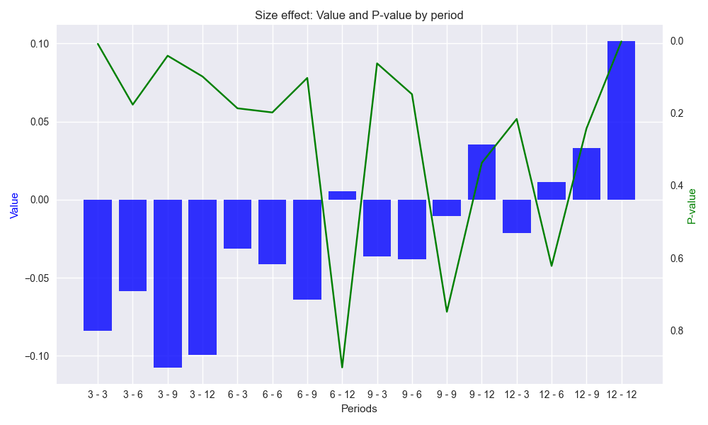
We’ll use the same periodic numbers – namely, 3, 6, 9, and 12 – for the weeks and test out all the combinations. But first, to ensure we’re not snooping our test period, we run the code only on the period up to, but excluding, 2019. We show a bar and line graph of the size effect and p-values of that size effect for the look forward period regressed against the lookback period returns. Note: we reverse the order of the p-values so that low p-values match larger size effects. Tomorrow we’ll discuss these results in more detail.

Code below.

# Built using Python 3.10.19 and a virtual environment 

# Load libraries
import pandas as pd
import numpy as np
from datetime import datetime, timedelta
import statsmodels.api as sm
import matplotlib.pyplot as plt
from matplotlib.ticker import FuncFormatter

plt.style.use('seaborn-v0_8')
plt.rcParams['figure.figsize'] = (14,8)

# Load data
df = yf.download('SPY', start='2000-01-01', end='2024-10-01')
df.columns = ['open', 'high', 'low', 'close', 'adj close', 'volume']
df.index.name = 'date'

# Create training set and downsample to weekly ending Friday
df_train = df.loc[:'2019-01-01', 'adj close'].copy()
df_w = pd.DataFrame(df_train.resample('W-FRI').last())
df_w.columns = ['price'] 

# Iterate through lookback and look forward periods
periods = [3, 6, 9, 12]
momo_dict = {}
for back in periods:
    for forward in periods:
        df_out = df_w.copy()
        df_out['ret_back'] = np.log(df_out['price']/df_out['price'].shift(back))
        df_out['ret_for'] = np.log(df_out['price'].shift(-forward)/df_out['price'])
        df_out = df_out.dropna()

        mod = sm.OLS(df_out['ret_for'], sm.add_constant(df_out['ret_back'])).fit()
        momo_dict[f"{back} - {forward}"] = {'data': df_out,
                                            'params': mod.params,
                                            'pvalues': mod.pvalues}

# Create Results data frame
df_results = pd.DataFrame({'periods': [key for key in momo_dict.keys()],
              'beta': [momo_dict[key]['params']['ret_back'] for key in momo_dict],
              'alpha': [momo_dict[key]['params']['const'] for key in momo_dict],
              'beta_pvalue': [momo_dict[key]['pvalues']['ret_back'] for key in momo_dict],
              'alpha_pvalue': [momo_dict[key]['pvalues']['const'] for key in momo_dict]
              })

# Create function to graph bar and line chart
def bar_and_line_plot(data: pd.DataFrame, x_var: str, y_bar: str, y_line: str,
                      y_bar_lab: str = 'Value', y_line_lab: str = 'P-value', 
                      title: str = 'Size effect', save_fig: bool = False, 
                      fig_title: str = 'size_effect_p_value',  ) -> None:
    fig, ax1 = plt.subplots(figsize=(10, 6))

    # Use datetime if available, else use numeric index
    x_axis = data[x_var]

    # Plot the area for the number of trades (background)
    ax1.bar(x_axis, data[y_bar], color='blue', label=y_bar_lab, alpha=0.8)
    ax1.set_xlabel('Periods')
    ax1.set_ylabel(y_bar_lab, color='blue')

    # Overlay the cumulative win rate (line plot)
    ax2 = ax1.twinx()  # Create a secondary y-axis for the win rate
    ax2.plot(x_axis, df_results[y_line], color='green', label=y_line_lab)
    ax2.set_ylabel(y_line_lab, color='green')
    ax2.invert_yaxis()

    # Add titles and grid
    plt.title(f"{title}: {y_bar_lab} and {y_line_lab} by period")
    ax2.grid()

    fig.tight_layout()

    if save_fig:
        plt.savefig(f"{title.lower()}_{fig_title}.png")
    plt.show()

# Graph size effects and p-values
bar_and_line_plot(df_results, 'periods', 'beta', 'beta_pvalue', save_fig=True)