Day 12: Iteration
In Day 11, we presented an initial iteration of train/forecast steps to see if one combination performs better than another. Our metric of choice was root mean-squared error (RMSE)1 which is frequently used to compare model performance in machine learning circles. The advantage of RMSE is that it is in the same units as the forecast variable. The drawback is that it is tough to interpret on its own. A model with a RMSE of 10 is better than one with 20. But what if the average actual value is one? Both are crap! Whatever the case, we can choose a more refined metric in the future, but RMSE is fine for now. As we saw, RMSE declines when you increase the training period up to a point and then rises again.
The causes of this variance were not clear. But should we spend more time trying to figure it out? Recall we have 16 different models. So wouldn’t it be more interesting to try all the train/forecast step combinations with all the momentum model combinations totaling 320 different iterations? Please say “Yes!” Although running such a test really doesn’t stress most computers, the process is not instantaneous.2 Nonetheless, we still think it’s pretty cool to imagine a bunch of combinations we’d like to test, have the computer chug through, after which we can analyze the results. Way cooler than creating sensitivity tables in Excel!
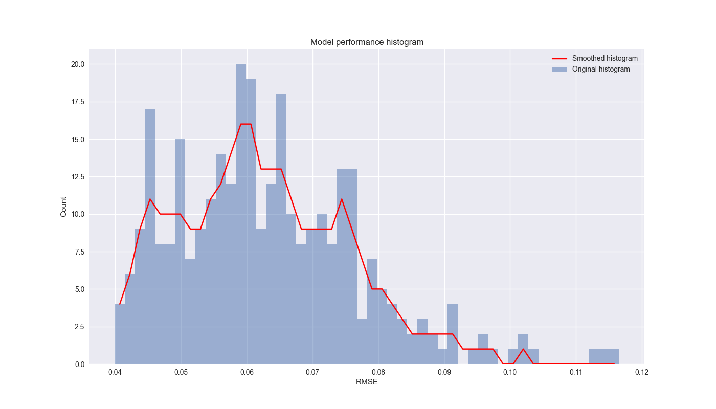
So let’s see what the results look like. To be sure, it will be hard to show the performance of 320 different model and walk-forward combinations. Instead, we graph a regular and smoothed histogram of the RMSEs below.

Notice that the mean is around 6% (the peak of the histogram) and that there is a positive skew, not just because RMSE does not take on negative values, but also because there are a few combinations that are really bad. We clipped the graph to remove some of those outliers.
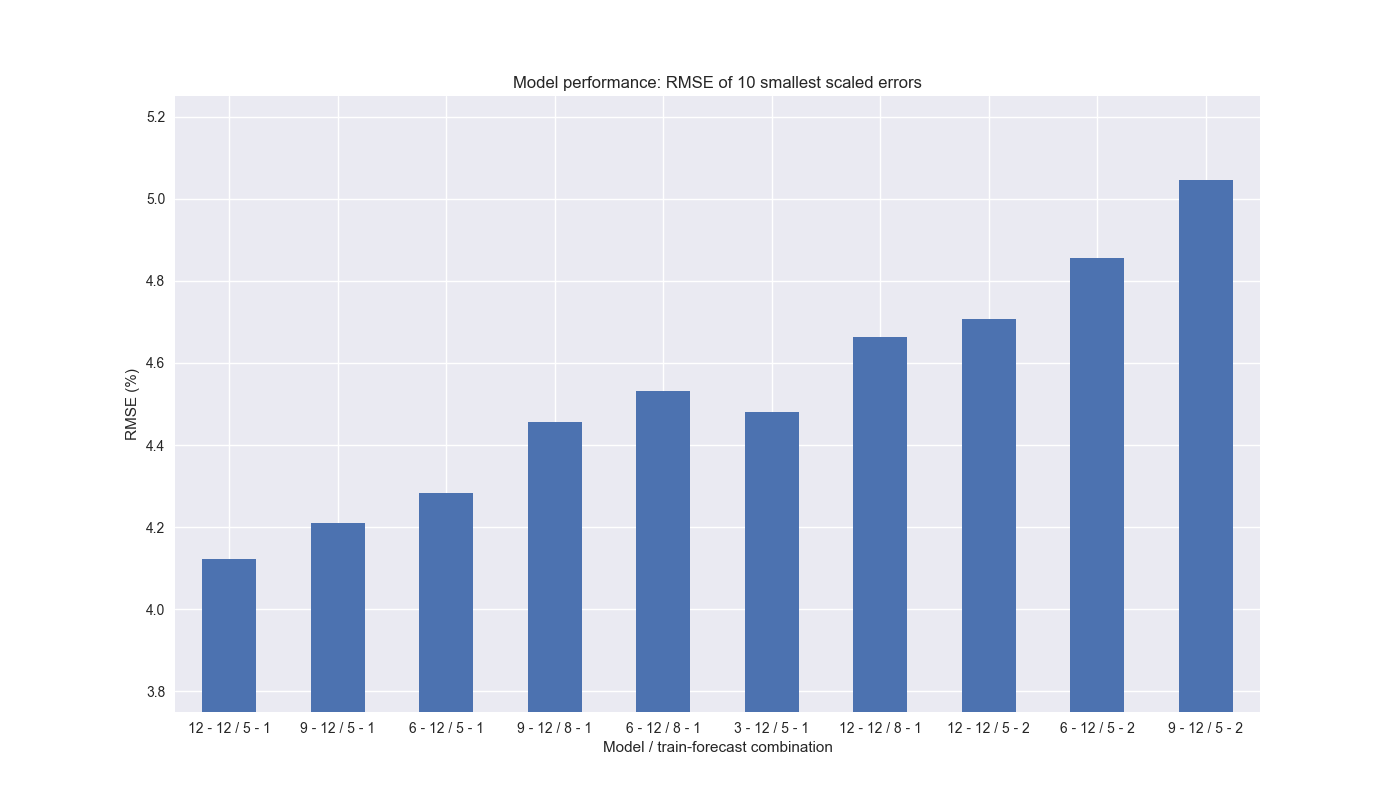
Now, let’s apply a scaling factor3 to the RMSE to further filter the results and graph the RMSE’s of the lowest 10 models based on this scaled factor with their combinations.

The model lookback periods are relatively uniform in frequency, except for the 3-week, which only appears once. However, all ten of the models use a 12-week look forward. A five step training period appears about 70% of the time with 8 steps the remainder. A one step forward forecast is the most prevalent. There are no other training periods represented. What is interesting is that the model performance decreases (RMSE goes up) as lookback period declines and/or model building period increases. The length of the forecast period does not seem as relevant. One should note that the difference in RMSE’s of these 10 models is relatively small – we’ve fiddled with the y-axis scale to heighten the differences.
On this analysis, it seems we should at least use a twelve week look forward for momentum and a 5/1 training/forecast step window. We’re particularly curious about the 3-12/5-1 model as it implies 3-week lookbacks appear to forecast 12-week look forwards pretty well, which is somewhat counter-intuitive. Since the 12-by-12/5-by-1 combination features the lowest RMSE, we’ll turn that into a trading signal in our next post. Code below.
# Built using Python 3.10.19 and a virtual environment

# Load libraries
import pandas as pd
import numpy as np
from datetime import datetime, timedelta
import statsmodels.api as sm
import matplotlib.pyplot as plt
from matplotlib.ticker import FuncFormatter
import yfinance as yf
from tqdm import tqdm
from scipy.ndimage import gaussian_filter1d

plt.style.use('seaborn-v0_8')
plt.rcParams['figure.figsize'] = (14,8)

# Function to get data
def get_spy_weekly_data() -> pd.DataFrame:
    df = yf.download('SPY', start='2000-01-01', end='2024-10-01')
    df.columns = ['open', 'high', 'low', 'close', 'adj close', 'volume']
    df.index.name = 'date'

    # Create training set and downsample to weekly ending Friday
    df_train = df.loc[:'2019-01-01', 'adj close'].copy()
    df_w = pd.DataFrame(df_train.resample('W-FRI').last())
    df_w.columns = ['price']

    return df_w

# Get data
df_w = get_spy_weekly_data()

# Create momentum dictionary
periods = [3, 6, 9, 12]
momo_dict = {}
for back in periods:
    for forward in periods:
        df_out = df_w.copy()
        df_out['ret_back'] = np.log(df_out['price']/df_out['price'].shift(back))
        df_out['ret_for'] = np.log(df_out['price'].shift(-forward)/df_out['price'])
        df_out = df_out.dropna()

        mod = sm.OLS(df_out['ret_for'], sm.add_constant(df_out['ret_back'])).fit()
        momo_dict[f"{back} - {forward}"] = {'data': df_out,
                                            'params': mod.params,
                                            'pvalues': mod.pvalues}

# Create models and parameters to iterate 320 different combinations
models = [x for x in momo_dict.keys()]
train_pds = [3, 5, 8, 13, 21]
test_pds = [1, 2, 3, 4]

# Instantiate dataframe to hold results and count
df_pd = pd.DataFrame(columns=['model', 'combo', 'rmse', 'rmse_scaled'])
count = 0

# Run iteration
for m in tqdm(models, desc="Models"):
    test = momo_dict[m]['data']
    for i in train_pds:
        for j in test_pds:
            tot_pd = i + j
            actual = []
            predicted = []
            for k in tqdm(range(tot_pd, len(test), j), desc="Walk forward", leave=False):
                train_df = test.iloc[k-tot_pd:k-j, 1:]
                test_df = test.iloc[k-j:k, 1:]

                # Ensure 'ret_back' is 2D by selecting it as a DataFrame, not a Series
                X_train = sm.add_constant(train_df[['ret_back']])
                if test_df.shape[0] > 1:
                    X_test = sm.add_constant(test_df[['ret_back']])
                else:
                    X_test = sm.add_constant(test_df[['ret_back']], has_constant='add')

                # Fit the model
                mod_run = sm.OLS(train_df['ret_for'], X_train).fit()

                # Predict using the test data
                mod_pred = mod_run.predict(X_test).values
                test_act = test_df['ret_for'].values
                predicted.extend(np.array(mod_pred))
                actual.extend(np.array(test_act))

            pred = np.array(predicted)
            act = np.array(actual)
            rmse = np.sqrt(np.mean((act - pred)**2))
            rmse_scaled = rmse / act.mean()
            df_pd.loc[count] = [m, f"{i} - {j}", rmse, rmse_scaled]
            count += 1

# Create a smoothed histogram function
def plot_smooth_hist(series: pd.Series | np.ndarray, bins: int = 50, xlab: str = 'RMSE',
                     title: str = "Model performance histogram", save_fig: bool = False,
                     fig_name: str = 'rmse_combo') -> None:

    counts, bin_edges = np.histogram(series, bins=bins)

    # Apply a Gaussian filter to the histogram counts to smooth it
    smoothed_counts = gaussian_filter1d(counts, sigma=1)

    # Plot the original histogram and the smoothed version
    bin_centers = 0.5 * (bin_edges[1:] + bin_edges[:-1])

    plt.bar(bin_centers, counts, width=bin_edges[1] - bin_edges[0], alpha=0.5, label='Original histogram')
    plt.plot(bin_centers, smoothed_counts, label='Smoothed histogram', color='red')
    plt.xlabel(xlab)
    plt.ylabel('Count')

    plt.legend()
    plt.title(title)
    if save_fig:
        plt.savefig(f"images/{fig_name}.png")
    plt.show()

# Plot smoothed histogram of RMSEs
plot_smooth_hist(df_pd['rmse'][df_pd['rmse']<0.12], save_fig=True, fig_name="rmse_combo_clipped")

# Add combination string to dataframe
df_pd['mod_combo'] = df_pd['model'] + " / " + df_pd['combo']

# Plot RMSEs of top ten smallest scaled RMSEs
(df_pd.nsmallest(10, 'rmse_scaled').set_index('mod_combo')['rmse']*100).plot(kind='bar', rot=0)
plt.ylim(3.75, 5.25)
plt.ylabel('RMSE (%)')
plt.xlabel("Model / train-forecast combination")
plt.title("Model performance: RMSE of 10 smallest scaled errors")
# plt.savefig("images/ten_smallest_models.png")
plt.show()

# Print the frequency of various combinations

# Lookback
print(df_pd.nsmallest(10, 'rmse_scaled')['model'].apply(lambda x: float(x[:2])).value_counts())

# Look forward
print(df_pd.nsmallest(10, 'rmse_scaled')['model'].apply(lambda x: float(x[-2:])).value_counts())

# Train step
print(df_pd.nsmallest(10, 'rmse_scaled')['combo'].apply(lambda x: float(x[:1])).value_counts())

# Forecast step
print(df_pd.nsmallest(10, 'rmse_scaled')['combo'].apply(lambda x: float(x[-1:])).value_counts())