Day 15: Backtest II

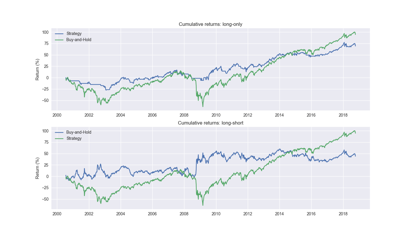
On Day 14 we showed how the trading model we built was snooping and provided one way to correct it. Essentially, we ensure the time in which we actually have the target variable data aligns with when the trading signals are produced. We then used the value of the next time step to input into the model to generate a forecast. If the forecast was positive, we’d go long the SPY ETF, if negative stay out of the market or short depending on the strategy. Results were decidedly worse than the snooped model. But, compared to buy-and-hold, they were not poop the bed horrible, though still underperforming. To refresh our memories, we plot the cumulative graph again below.

The strategy underperforms buy-and-hold by about 25% points. However, its Sharpe Ratio is about 600bps higher at 36% – nice, but nothing to write home about. We’ll forego a broader analysis as we presented on Day 3. Some readers may be wondering why the heck would you use the time stamp directly after the last training step when it’s clearly 11 weeks old? Glad you asked. It does indeed seem stale at best, silly at worst. We wanted to show it for completeness of comparison. A likely better input is the most recent time stamp. That is, the model is trained on lookback returns whose forward returns are indeed 12-weeks ahead, as opposed those that mostly already occurred. When we finally get to that 12th week to train the model, we can turnaround and use the lookback data from the most recently completed week to input into the model to generate a prediction.

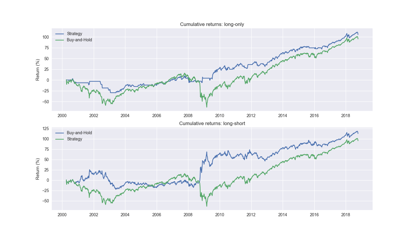
Let’s do that now and graph the result below.

Certainly more of the result we were looking for! Here the long-only strategy outperforms buy-and-hold by 10% points. Long-short is even better. Critically, long-only’s Sharpe Ratio is over 20% points higher; long-short’s is about 600bps better. This definitely warrants further investigation and comparison to our benchmarks, which delve into tomorrow.Stay tuned!

Code below.

# Built using Python 3.10.19 and a virtual environment 

# Load libraries
import pandas as pd
import numpy as np
from datetime import datetime, timedelta
import statsmodels.api as sm
import matplotlib.pyplot as plt
import yfinance as yf

plt.style.use('seaborn-v0_8')
plt.rcParams['figure.figsize'] = (14,8)

# Function to get data
def get_spy_weekly_data() -> pd.DataFrame:
    df = yf.download('SPY', start='2000-01-01', end='2024-10-01')
    df.columns = ['open', 'high', 'low', 'close', 'adj close', 'volume']
    df.index.name = 'date'

    # Create training set and downsample to weekly ending Friday
    df_train = df.loc[:'2019-01-01', 'adj close'].copy()
    df_w = pd.DataFrame(df_train.resample('W-FRI').last())
    df_w.columns = ['price'] 

    return df_w

# Get data
df_w = get_spy_weekly_data()

# Create momentum dictionary
periods = [3, 6, 9, 12]
momo_dict = {}
for back in periods:
    for forward in periods:
        df_out = df_w.copy()
        df_out['ret_back'] = np.log(df_out['price']/df_out['price'].shift(back))
        df_out['ret_for'] = np.log(df_out['price'].shift(-forward)/df_out['price'])
        df_out = df_out.dropna()

        mod = sm.OLS(df_out['ret_for'], sm.add_constant(df_out['ret_back'])).fit()
        momo_dict[f"{back} - {forward}"] = {'data': df_out,
                                            'params': mod.params,
                                            'pvalues': mod.pvalues}

# Prepare model
model_name = '12 - 12'
mod_look_forward = 12
train_pd = 5
test_pd = 1
tot_pd = train_pd + test_pd

# Create trading dataframe
df_trade = momo_dict[model_name]['data'].copy()

# Run model with train/forecast steps
trade_pred = []
for i in range(tot_pd, len(df_trade)+1, test_pd):
    train_df = df_trade.iloc[i-tot_pd:i-test_pd, 1:]
    test_df = df_trade.iloc[i-test_pd+mod_look_forward-1:i-test_pd+mod_look_forward, 1:]

    # Ensure 'ret_back' is 2D by selecting it as a DataFrame, not a Series
    X_train = sm.add_constant(train_df[['ret_back']])
    if test_df.shape[0] > 1:
        X_test = sm.add_constant(test_df[['ret_back']])
    else:
        X_test = sm.add_constant(test_df[['ret_back']], has_constant='add')

    # Fit the model
    mod_run = sm.OLS(train_df['ret_for'], X_train).fit()

    # Predict using the test data
    mod_pred = mod_run.predict(X_test).values
    trade_pred.extend(mod_pred)

# Add predictions to dataframe
# Snooped predictions. Pad = train_pd
# df_trade['pred'] = np.concatenate((np.repeat(np.nan,train_pd), np.array(trade_pred)))

# Non-snooped. Pad = mod_look_forward + train_pd
# Same as in Day 14 but test_df is moved forward in for loop
df_trade['pred'] = np.concatenate((np.repeat(np.nan, mod_look_forward + train_pd - 1), np.array(trade_pred[:-(mod_look_forward - 1)])))

# Generate returns
df_trade['ret'] = np.log(df_trade['price']/df_trade['price'].shift(1))

# Generate signals
df_trade['signal'] = np.where(df_trade['pred'] == np.nan, np.nan, np.where(df_trade['pred'] > 0, 1, 0))
df_trade['signal_sh'] = np.where(df_trade['pred'] == np.nan, np.nan, np.where(df_trade['pred'] >= 0, 1, -1))

# Generate strategy returns
df_trade['strat_ret'] = df_trade['signal'].shift(1) * df_trade['ret']
df_trade['strat_ret_sh'] = df_trade['signal_sh'].shift(1) * df_trade['ret']

# Plot cumulative performance plot for long-only and long-short
fig, (ax1, ax2) = plt.subplots(2,1)

top = df_trade[['strat_ret_snoop', 'ret']].cumsum()
bottom = df_trade[['strat_ret_snoop_sh', 'ret']].cumsum()

ax1.plot(top.index, top.values*100)
ax1.set_xlabel("")
ax1.set_ylabel("Return (%)")
ax1.legend(['Strategy', 'Buy-and-Hold'], loc="upper left")
ax1.set_title("Cumulative returns: long-only")

ax2.plot(bottom.index, bottom.values*100)
ax2.set_xlabel("")
ax2.set_ylabel("Return (%)")
ax2.legend(['Strategy', 'Buy-and-Hold'], loc="upper left")
ax2.set_title("Cumulative returns: long-short")

plt.show()