Day 16: Comps
On Day 15 we adjusted our model to use more recent data to forecast the 12-week look forward return. As before, we used that forecast to generate a trading signal that tells us to go long the SPY if the forecast is positive, and exit (or short for the long-short strategy) if otherwise. We saw this tweak generated about 10% points of cumulative outperformance and a 20% point higher Sharpe Ratio. We’ll now return to the performance metrics and tearsheet we first introduced on Day 3
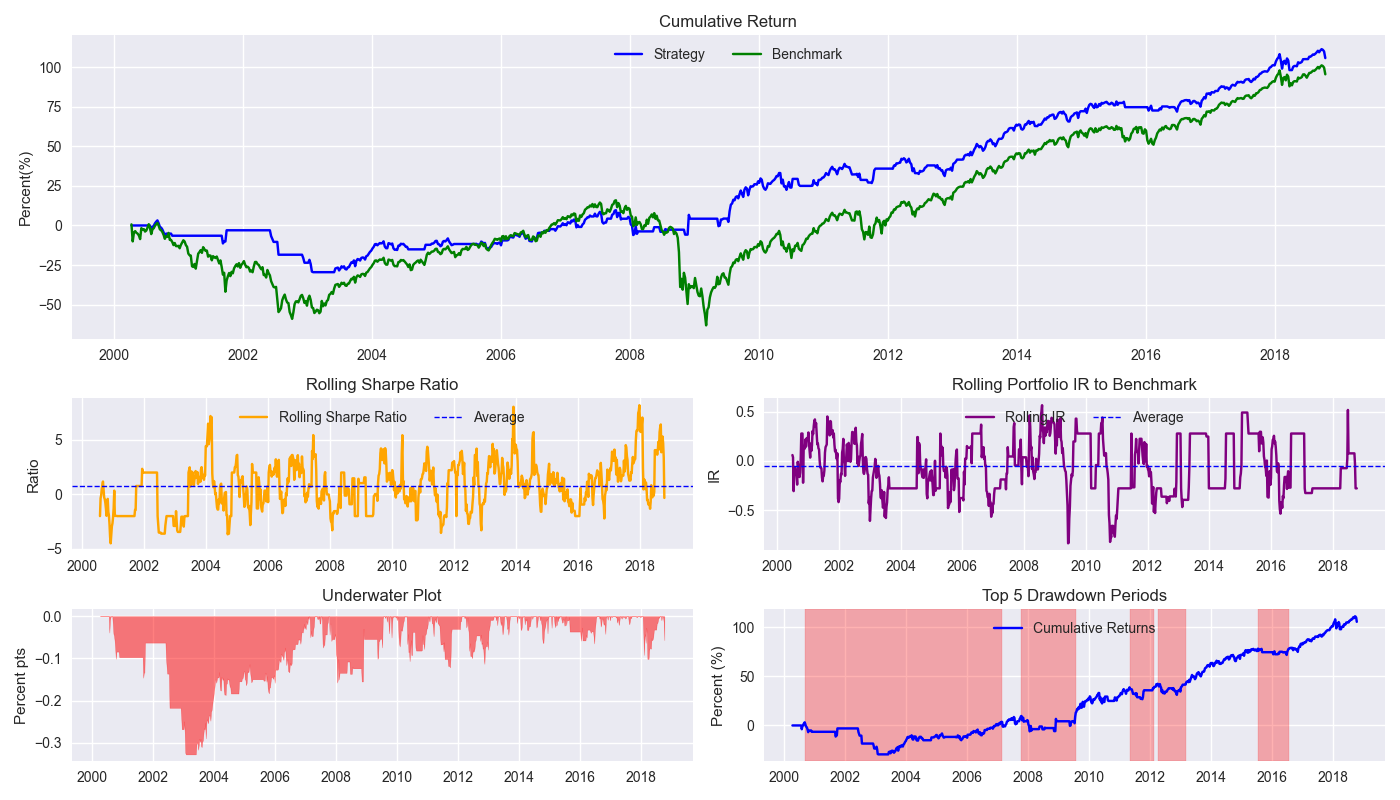
Let’s first compare the performance of the strategy relative to buy-and-hold. We’ve already shown the cumulative performance chart, but now we include the other charts. The strategy successfully keeps one out of the 2002-2003 bottom as well as most of the global financial crisis and generally captures the upward trend of the underlying market during the rest of the time. The 8-week rolling Sharpe ratio shows some pretty substantial choppiness. That said, it does not appear to be declining over time. The rolling Information Ratio (IR) also exhibits similar choppiness. While it does spike above 0.5 on occasion (generally indicating a pretty good strategy), the overall ratio is pretty much close to zero. We should note that the IR is not particularly relevant in this case since there’s no security selection involved – that is, we’re not over or underweighting different securities relative to the index.

Let’s turn to drawdowns. We note that the max drawdown occurred in late 2003 with a greater than 30% peak-to-trough decline. This compares with buy-and-hold, which suffered a more than 55% decline in the same period. Of the top 5 drawdown periods, the 2000 to 2007 is the longest and would certainly be difficult to endure even if the market is performing worse. Let’s turn to the other benchmarks. First, the 60-40 portfolio below.

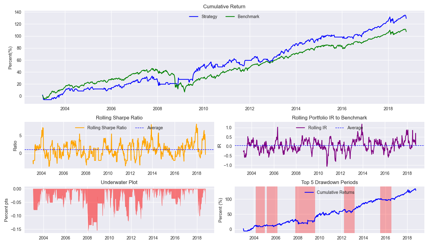
Compared to the SPY-IEF 60-40 quarterly rebalanced benchmark, the strategy performs quite nicely, outperforming by a cumulative 22% points. How’s your investment advisor doing with those 60-40 recommendations? Drop us an email and we’ll send you our ADV ASAP. We’re joking of course. This is for educational purposes only. Note: the underwater plot is different because IEF data was not available for much of the 2000-2003 timeframe so that is removed from the comparison set.
How about the 200-day SMA?

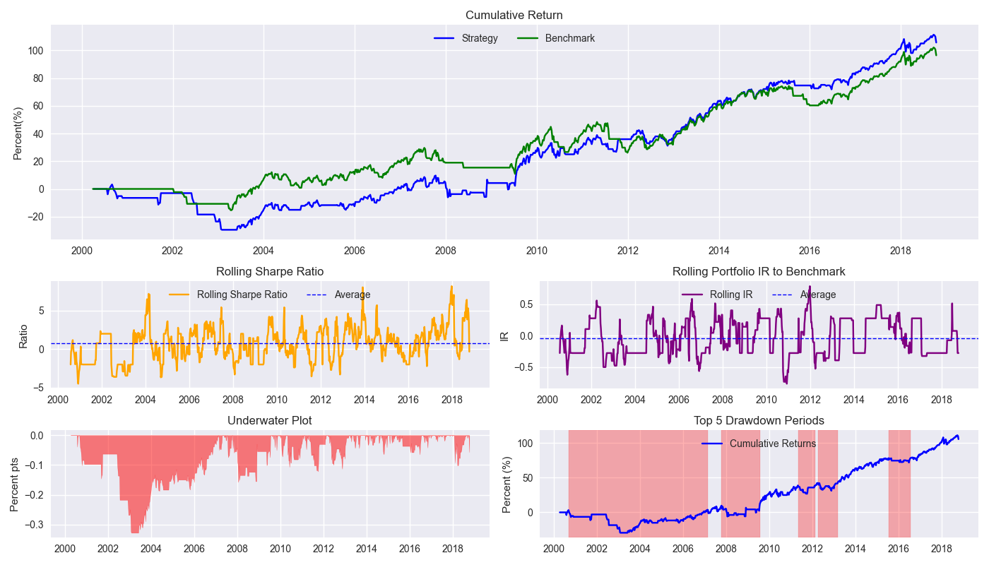
Interestingly, the 200-day SMA outperforms the 12-by-12 for most of the period except for 2015-2018 period. And it is that period that leads to the 12-by-12 exceeding the 200-day SMA by about a 10% points on a cumulative return basis. The differences in the Sharpe ratio are de minimis.
We’ll have more to say about these comparisons in our next post.
Code below.
# Built using Python 3.10.19 and a virtual environment

# Load libraries
import pandas as pd
import numpy as np
from datetime import datetime, timedelta
import statsmodels.api as sm
import matplotlib.pyplot as plt
from matplotlib.ticker import FuncFormatter
import matplotlib as mpl
from matplotlib.gridspec import GridSpec
from scipy.stats import linregress
import yfinance as yf

plt.style.use('seaborn-v0_8')
plt.rcParams['figure.figsize'] = (14,8)

# Function to get data
def get_spy_weekly_data() -> pd.DataFrame:
    df = yf.download('SPY', start='2000-01-01', end='2024-10-01')
    df.columns = ['open', 'high', 'low', 'close', 'adj close', 'volume']
    df.index.name = 'date'

    # Create training set and downsample to weekly ending Friday
    df_train = df.loc[:'2019-01-01', 'adj close'].copy()
    df_w = pd.DataFrame(df_train.resample('W-FRI').last())
    df_w.columns = ['price']

    return df_w

# Get data
df_w = get_spy_weekly_data()

# Create momentum dictionary
periods = [3, 6, 9, 12]
momo_dict = {}
for back in periods:
    for forward in periods:
        df_out = df_w.copy()
        df_out['ret_back'] = np.log(df_out['price']/df_out['price'].shift(back))
        df_out['ret_for'] = np.log(df_out['price'].shift(-forward)/df_out['price'])
        df_out = df_out.dropna()

        mod = sm.OLS(df_out['ret_for'], sm.add_constant(df_out['ret_back'])).fit()
        momo_dict[f"{back} - {forward}"] = {'data': df_out,
                                            'params': mod.params,
                                            'pvalues': mod.pvalues}

# Prepare model
model_name = '12 - 12'
mod_look_forward = 12
train_pd = 5
test_pd = 1
tot_pd = train_pd + test_pd

# Create trading dataframe
df_trade = momo_dict[model_name]['data'].copy()

# Run model with train/forecast steps
trade_pred = []
for i in range(tot_pd, len(df_trade)+1, test_pd):
    train_df = df_trade.iloc[i-tot_pd:i-test_pd, 1:]
    test_df = df_trade.iloc[i-test_pd+mod_look_forward-1:i-test_pd+mod_look_forward, 1:]

    # Ensure 'ret_back' is 2D by selecting it as a DataFrame, not a Series
    X_train = sm.add_constant(train_df[['ret_back']])
    if test_df.shape[0] > 1:
        X_test = sm.add_constant(test_df[['ret_back']])
    else:
        X_test = sm.add_constant(test_df[['ret_back']], has_constant='add')

    # Fit the model
    mod_run = sm.OLS(train_df['ret_for'], X_train).fit()

    # Predict using the test data
    mod_pred = mod_run.predict(X_test).values
    trade_pred.extend(mod_pred)

# Add predictions to dataframe
df_trade['pred'] = np.concatenate((np.repeat(np.nan, mod_look_forward + train_pd - 1), np.array(trade_pred)))

# Generate returns
df_trade['ret'] = np.log(df_trade['price']/df_trade['price'].shift(1))

# Generate signals
df_trade['signal'] = np.where(df_trade['pred'] == np.nan, np.nan, np.where(df_trade['pred'] > 0, 1, 0))
df_trade['signal_sh'] = np.where(df_trade['pred'] == np.nan, np.nan, np.where(df_trade['pred'] >= 0, 1, -1))

# Generate strategy returns
df_trade['strat_ret'] = df_trade['signal'].shift(1) * df_trade['ret']
df_trade['strat_ret_sh'] = df_trade['signal_sh'].shift(1) * df_trade['ret']

# Load data for benchmarks
data = yf.download(['SPY', 'IEF'], start='2000-01-01', end='2024-10-01')
df = data.loc["2003-01-01":, 'Adj Close']
df.columns.name = None
tickers = ['ief', 'spy']
df.index.name = 'date'
df.columns = tickers
df[['ief_chg', 'spy_chg']] = df[['ief','spy']].apply(lambda x: np.log(x/x.shift(1)))
df_bw =  pd.DataFrame(df.resample('W-FRI').last())
df_bw[['ief_chg', 'spy_chg']] = df_bw[['ief','spy']].apply(lambda x: np.log(x/x.shift(1)))

# Align dates for comparisons
end_date_bench = df_trade.index[-1].strftime("%Y-%m-%d")
bench_returns = df_bw[['ief_chg', 'spy_chg']].copy()
bench_returns = bench_returns.loc[:end_date_bench]
bench_returns = bench_returns.dropna()

strat_returns_start = bench_returns.index[0].strftime("%Y-%m-%d")
strat_returns = df_trade['strat_ret'].copy()
strat_returns = strat_returns.loc[strat_returns_start:]

# Create function to calculate portfolio performance
def calculate_portfolio_performance(weights: list, returns: pd.DataFrame, rebalance=False, frequency='month') -> pd.Series:
    # Initialize the portfolio value to 0.0
    portfolio_value = 0.0
    portfolio_values = []

    # Initialize the current weights
    current_weights = np.array(weights)

    # Create a dictionary to map frequency to the appropriate offset property
    frequency_map = {
        'week': 'week',
        'month': 'month',
        'quarter': 'quarter'
    }

    if rebalance:
        # Iterate over each row in the returns DataFrame
        for date, daily_returns in returns.iterrows():
            # Apply the current weights to the daily returns
            portfolio_value = np.dot(current_weights, daily_returns)
            portfolio_values.append(portfolio_value)

            # Rebalance at the selected frequency (week, month, quarter)
            offset = pd.DateOffset(days=1)
            next_date = date + offset #type: ignore

            # Dynamically get the attribute based on frequency
            current_period = getattr(date, frequency_map[frequency])
            next_period = getattr(next_date, frequency_map[frequency])

            # If current period does not equal next period, time to rebalance
            if current_period != next_period:
                current_weights = np.array(weights)
            else:
                # Update weights based on the previous day's returns
                current_weights = current_weights * (1 + daily_returns)
                current_weights /= np.sum(current_weights)
    else:
        # No rebalancing, just apply the initial weights
        for date, daily_returns in returns.iterrows():
            portfolio_value = np.dot(current_weights, daily_returns)
            portfolio_values.append(portfolio_value)

            # Update weights based on the previous day's returns
            current_weights = current_weights * (1 + daily_returns)
            current_weights /= np.sum(current_weights)

    daily_returns = pd.Series(portfolio_values, index=returns.index)

    return daily_returns

# Create 60-40 portfolio
weights = [0.4,0.6]
bench_60_40_rebal = calculate_portfolio_performance(weights, bench_returns, rebalance=True, frequency='quarter')
bench_60_40_rebal.index = bench_60_40_rebal.index.tz_localize(None) #type:ignore

# Create 200-day strategy
df_200 = df_w.copy()
df_200.columns = ['price']
df_200 = df_200.resample('W-FRI').last()
# 40 weeks = 200 days
df_200['sma_200'] = df_200['price'].rolling(40).mean()
df_200['ret'] = np.log(df_200['price']/df_200['price'].shift(1))
df_200['signal'] = np.where(df_200['price'] > df_200['sma_200'], 1, 0)
df_200['strat_ret'] = df_200['signal'].shift(1)*df_200['ret']
df_200_bench = df_200.loc[df_trade['strat_ret'].index[0]:df_trade['strat_ret'].index[-1]]

# Create functions for tearsheet plot
# Rolling beta
def rolling_beta(portfolio_returns, market_returns, window=60, assume=True, threshold=2.0):
    def get_beta_coef(x_var, y_var):
        if assume:
            # coeffs = np.linalg.lstsq(x_var.values[:,np.newaxis], y_var)[0]
            coeffs = np.linalg.lstsq(np.vstack(x_var), y_var)[0]
            coeffs = coeffs if np.abs(coeffs) <= threshold else np.sign(coeffs)*threshold
            return coeffs[0]
        else:
            coeffs = np.linalg.lstsq(np.vstack([x_var, np.ones(len(x_var))]).T, y_var)[0]
            coeffs = coeffs if np.abs(coeffs) <= threshold else np.sign(coeffs)*threshold
            return coeffs[0]
    return portfolio_returns.rolling(window).apply(lambda x: get_beta_coef(x, market_returns.loc[x.index]))

# Rolling information ratio
def rolling_ir(portfolio_returns, market_returns, window=60):
    def get_tracking_error(portfolio, benchmark):
        return (portfolio - benchmark).std()
    return portfolio_returns.rolling(window).apply(lambda x: (x.mean() - market_returns.loc[x.index].mean())/get_tracking_error(x, market_returns.loc[x.index]))

# Define a function to calculate rolling Sharpe ratio
def rolling_sharpe_ratio(returns, window=60, period=252):
    rolling_sharpe = returns.rolling(window).mean() / returns.rolling(window).std() * np.sqrt(period)
    return rolling_sharpe

# Define a function to calculate drawdowns and identify drawdown periods
def get_drawdown_periods(cumulative_returns):
    peak = cumulative_returns.cummax()
    drawdown = cumulative_returns - peak

    end_of_dd = drawdown[drawdown == 0].index
    dd_periods = []
    start = cumulative_returns.index[0]
    for end in end_of_dd:
        if start < end:
            period = (start, end)
            dd_periods.append(period)
        start = end

    return drawdown, dd_periods

# Define a function to plot drawdowns
def plot_drawdowns(cumulative_returns):
    drawdown, dd_periods = get_drawdown_periods(cumulative_returns)
    dd_durations = [(end - start).days for start, end in dd_periods]
    top_dd_periods = sorted(dd_periods, key=lambda x: (x[1] - x[0]).days, reverse=True)[:5]
    return drawdown, top_dd_periods

# Plot tearsheet
def plot_tearsheet(portfolio_returns, market_returns, window=60, period=252, save_figure=False, title=None):
    cumulative_portfolio_returns = portfolio_returns.cumsum()
    cumulative_market_returns = market_returns.cumsum()

    fig = plt.figure(figsize=(14, 8))
    gs = GridSpec(3, 2, height_ratios=[2, 1, 1], width_ratios=[1, 1])

    # Cumulative return with no rebalancing plot
    ax0 = fig.add_subplot(gs[0, :])
    ax0.plot(cumulative_portfolio_returns*100, label='Strategy', color='blue')
    ax0.plot(cumulative_market_returns*100, label='Benchmark', color='green')
    ax0.legend(loc='upper center', ncol=2)
    ax0.set_title('Cumulative Return')
    ax0.set_ylabel('Percent(%)')

    # Rolling Sharpe ratio plot
    ax1 = fig.add_subplot(gs[1, 0])
    rolling_sr = rolling_sharpe_ratio(portfolio_returns, window=window, period=period)
    rolling_sr = rolling_sr.ffill()
    ax1.plot(rolling_sr, color='orange', label='Rolling Sharpe Ratio')
    ax1.axhline(rolling_sr.mean(), color='blue', ls='--', lw=1, label='Average')
    ax1.legend(loc='upper center', ncol = 2)
    ax1.set_title('Rolling Sharpe Ratio')
    ax1.set_ylabel('Ratio')

    # Rolling Information ratio plot
    ax2 = fig.add_subplot(gs[1, 1])
    roll_ir = rolling_ir(portfolio_returns, market_returns, window=window)
    roll_ir = roll_ir.ffill()
    ax2.plot(roll_ir, color='purple', label='Rolling IR')
    ax2.axhline(roll_ir.mean(), color='blue', ls='--', lw=1, label='Average')
    ax2.legend(loc='upper center', ncol = 2)
    ax2.set_title('Rolling Portfolio IR to Benchmark')
    ax2.set_ylabel('IR')

    # Underwater plot
    ax3 = fig.add_subplot(gs[2, 0])
    drawdown, top_dd_periods = plot_drawdowns(cumulative_portfolio_returns)
    ax3.fill_between(drawdown.index, drawdown, color='red', alpha=0.5)
    ax3.set_title('Underwater Plot')
    ax3.set_ylabel('Percent pts')

    # Top 5 drawdown periods plot
    ax4 = fig.add_subplot(gs[2, 1])
    for start, end in top_dd_periods:
        ax4.axvspan(start, end, color='red', alpha=0.3)
    ax4.plot(cumulative_portfolio_returns*100, label='Cumulative Returns', color='blue')
    ax4.legend(loc='upper center')
    ax4.set_title('Top 5 Drawdown Periods')
    ax4.set_ylabel('Percent (%)')

    plt.tight_layout()
    if save_figure:
        fig.savefig(f'images/{title}.png')

    plt.show()

# Plot tearsheet for strategy vs buy-and-hold
#. window=13 as 13 weeks ~3months, period=52 for sharpe annualization
plot_tearsheet(df_trade['strat_ret'], df_trade['ret'], window=13, period=52)

# Plot tearsheet for strategy vs 60-40
plot_tearsheet(strat_returns, bench_60_40_rebal, window=13, period=52)

# Plot tearsheet for strategy vs. 200-day
plot_tearsheet(df_trade['strat_ret'], df_200_bench['strat_ret'], window=13, period=52)