Day 26: Adjusted vs. Original

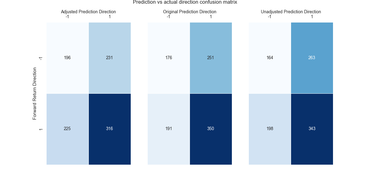
The last five days! On Day 25, we compared the peformance of the adjusted vs. unadjusted strategy for different prediction scenarios: true and false positives and negatives. For true positives and false negatives, the adjusted strategy performed better than the unadjusted. For true negatives and false positives, the unadjusted strategy performed better.  Today, we run the same comparisons with the original 12-by-12 strategy. We present the confusion matrices below for all three strategies.

In the case of the adjusted and original strategies above, we can see that the adjusted strategy has fewer true positives and more true negatives than the original strategy. This matches a similar result for the unadjusted strategy. The adjusted strategy has far fewer false positives at 231 than the original at 251, which is slightly lower than the unadjusted. However, the adjusted strategy has more false negatives than the original at 225 vs. 191, which is also less than the unadjusted. Interestingly, the original strategy also has more true positives and true negatives than the unadjusted.

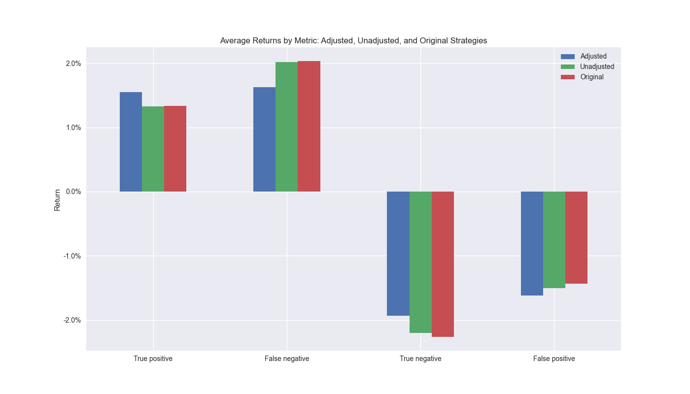
We’ll now look at average returns by prediction scenarios for all three strategies.

As one can see based on the true positives, the adjusted strategy has a higher average return than both the unadjusted and original strategies. The adjusted strategy also has a lower average return than either the unadjusted or original for false negatives, meaning that when it incorrectly predicts a down market, the strategy doesn’t suffer as much. On the true negative side, both the unadjusted and original strategies perform better. Finally, the adjusted strategy suffers a worse average return than the unadjusted or original strategies for false positives.

Based on these results we can make a few summary conclusions. The two major contributors to the success of the adjusted strategy appears to be getting more of the big moves correct and not missing the big moves when it is incorrect. This seems to work even if the total number of correct predictions are fewer than the competing strategies. Interestingly, even though the competing strategies were more adept at avoiding big negative moves, the greater frequency of correct true negatives might have offset that advantage. Another interesting observation is the relatively similarity in returns between the unadjusted and original strategies for the various prediction scenarios. Looking at such results would not lead one to expect the original strategy to outperform the unadjusted one. But it does likely because the higher frequency of true positives and true negatives, being higher than the unadjusted strategy, has some compounding effects that lead the original strategy outperform.

A final point that bears out our conclusions. When we run t-tests on the difference in means between the adjusted, unadjusted, and original strategies, we note that it is indeed the true positives and false negatives that show a significant difference between the adjusted and competing strategies based on p-values below the 0.05 threshold. Note the difference in mean returns between the unadjusted and original strategy are not significant, perhaps further supporting the argument that the higher frequency of correct results drove the performance of the original strategy.¹

		T-test P-values
	Adjusted vs. Unadjusted	Adjusted vs. Original	Unadjusted vs. Original
True positive	0.016	0.021	0.516
False negative	0.001	0.006	0.540
True negative	0.131	0.085	0.418
False positive	0.765	0.870	0.685

We have one final adjustment we want to make to the strategy and might yield even further performance enhancements. We’ll explore that in our next post. Stay tuned!

Code below.

# Built using Python 3.10.19 and a virtual environment 

# Load packages
import pandas as pd
import numpy as np
from datetime import datetime, timedelta
import statsmodels.api as sm
import matplotlib.pyplot as plt
from matplotlib.ticker import FuncFormatter
import yfinance as yf
import seaborn as sns
from scipy.stats import ttest_ind

plt.style.use('seaborn-v0_8')
plt.rcParams['figure.figsize'] = (14,8)

def get_spy_weekly_data() -> pd.DataFrame:
    df = yf.download('SPY', start='2000-01-01', end='2024-10-01')
    df.columns = ['open', 'high', 'low', 'close', 'adj close', 'volume']
    df.index.name = 'date'

    # Create training set and downsample to weekly ending Friday
    df_train = df.loc[:'2019-01-01', 'adj close'].copy()
    df_w = pd.DataFrame(df_train.resample('W-FRI').last())
    df_w.columns = ['price'] 

    return df_w

df_w = get_spy_weekly_data()

# Create momentum dictionary
periods = [3, 6, 9, 12]
momo_dict = {}
for back in periods:
    for forward in periods:
        df_out = df_w.copy()
        df_out['ret_back'] = np.log(df_out['price']/df_out['price'].shift(back))
        df_out['ret_for'] = np.log(df_out['price'].shift(-forward)/df_out['price'])
        df_out = df_out.dropna()

        mod = sm.OLS(df_out['ret_for'], sm.add_constant(df_out['ret_back'])).fit()
        momo_dict[f"{back} - {forward}"] = {'data': df_out,
                                            'params': mod.params,
                                            'pvalues': mod.pvalues}


# Trade with error handling
df_trade_1 = momo_dict['12 - 12']['data'].copy()

mod_look_forward = 12
train_pd = 5
test_pd = 1
tot_pd = train_pd + test_pd
lr = 2

trade_pred = []
trade_pred_un = []
trade_pred_old = []
for i in range(tot_pd, len(df_trade_1)-mod_look_forward+1, test_pd):
    train_df = df_trade_1.iloc[i-tot_pd:i-test_pd, 1:]
    valid_df = df_trade_1.iloc[i-test_pd:i, 1:]
    uncorr_df = df_trade_1.iloc[i-test_pd+mod_look_forward-1:i-test_pd+mod_look_forward, 1:]
    test_df = df_trade_1.iloc[i-test_pd+mod_look_forward:i-test_pd+mod_look_forward+1, 1:]

    # Ensure 'ret_back' is 2D by selecting it as a DataFrame, not a Series
    X_train = sm.add_constant(train_df[['ret_back']])
    if valid_df.shape[0] > 1:
        X_valid = sm.add_constant(valid_df[['ret_back']])
    else:
        X_valid = sm.add_constant(valid_df[['ret_back']], has_constant='add')

    if uncorr_df.shape[0] > 1:
        X_uncorr = sm.add_constant(uncorr_df[['ret_back']])
    else:
        X_uncorr = sm.add_constant(uncorr_df[['ret_back']], has_constant='add')

    if test_df.shape[0] > 1:
        X_test = sm.add_constant(test_df[['ret_back']])
    else:
        X_test = sm.add_constant(test_df[['ret_back']], has_constant='add')

    # Fit the model
    mod = sm.OLS(train_df['ret_for'], X_train).fit()

    # Predict using the test data
    pred = mod.predict(X_valid).values
    actual = valid_df['ret_for'].values
    gamma = -(actual - pred)*lr
    # gamma = -1 if np.sign(actual) + np.sign(pred) == 0 else 1
    pred_old = mod.predict(X_uncorr)
    trade_pred_old.extend(pred_old)

    mod_pred = mod.predict(X_test).values
    trade_pred_un.extend(mod_pred)
    trade_pred.extend(mod_pred + gamma)

assert len(trade_pred) + mod_look_forward + train_pd == len(df_trade_1)
assert len(trade_pred_un) + mod_look_forward + train_pd == len(df_trade_1)

df_trade_1['pred'] = np.concatenate((np.zeros(mod_look_forward + train_pd), np.array(trade_pred)))
df_trade_1['pred_un'] = np.concatenate((np.zeros(mod_look_forward + train_pd), np.array(trade_pred_un)))
df_trade_1['pred_old'] = np.concatenate((np.zeros(mod_look_forward + train_pd - 1), np.array(trade_pred_old), np.zeros(1)))
df_trade_1['ret'] = np.log(df_trade_1['price']/df_trade_1['price'].shift(1))

df_trade_1['signal'] = np.where(df_trade_1['pred'] > 0, 1, 0)
df_trade_1['signal_un'] = np.where(df_trade_1['pred_un'] > 0, 1, 0)
df_trade_1['signal_old'] = np.where(df_trade_1['pred_old'] > 0, 1, 0)
df_trade_1['signal_sh'] = np.where(df_trade_1['pred'] >= 0, 1, -1)

df_trade_1['strat_ret'] = df_trade_1['signal'].shift(1) * df_trade_1['ret']
df_trade_1['strat_ret_un'] = df_trade_1['signal_un'].shift(1) * df_trade_1['ret']
df_trade_1['strat_ret_old'] = df_trade_1['signal_old'].shift(1) * df_trade_1['ret']
df_trade_1['strat_ret_sh'] = df_trade_1['signal_sh'].shift(1) * df_trade_1['ret']


# Sign analysis
df_corr = df_trade_1[['pred', 'pred_un', 'pred_old', 'gamma', 'ret', 'ret_for', 'ret_back']].copy()

# Confusion matrices analysis
# Convert values to sign: -1 (negative), 0 (neutral), 1 (positive)
pred_sign = [1 if x == 1 else -1 for x in np.sign(df_corr['pred'])]
pred_un_sign = [1 if x == 1 else -1 for x in np.sign(df_corr['pred_un'])]
ret_sign = [1 if x == 1 else -1 for x in np.sign(df_corr['ret_lag'])]
pred_old_sign = [1 if x == 1 else -1 for x in np.sign(df_corr['pred_old'])]

# Create a DataFrame
pred_data = pd.DataFrame({'Prediction': pred_sign, 'Return': ret_sign})
pred_un_data = pd.DataFrame({'Prediction': pred_un_sign, 'Return': ret_sign})
pred_old_data = pd.DataFrame({'Prediction': pred_old_sign, 'Return': ret_sign})

# Create a heatmap of counts for each combination
pred_heatmap = pred_data.groupby(['Prediction', 'Return']).size().unstack(fill_value=0)
pred_un_heatmap = pred_un_data.groupby(['Prediction', 'Return']).size().unstack(fill_value=0)
pred_old_heatmap = pred_old_data.groupby(['Prediction', 'Return']).size().unstack(fill_value=0)

# Create heatmaps for percent
pred_heatmap_percent = pred_heatmap/pred_heatmap.values.sum()*100
pred_un_heatmap_percent = pred_un_heatmap/pred_un_heatmap.values.sum()*100
pred_old_heatmap_percent = pred_old_heatmap/pred_old_heatmap.values.sum()*100

# Create annotations
annot1 = pred_heatmap_percent.applymap(lambda x: f"{x:.1f}%").values
annot2 = pred_un_heatmap_percent.applymap(lambda x: f"{x:.1f}%").values
annot3 = pred_old_heatmap_percent.applymap(lambda x: f"{x:.1f}%").values

# Heatmap
fig, (ax1, ax2, ax3) = plt.subplots(1,3, sharey=True, figsize=(12,6))
fig.text(0.5, 0.98, "Prediction vs actual direction confusion matrix", ha='center', fontsize=12)

sns.heatmap(pred_heatmap.T, annot=True, fmt='d', cmap='Blues', cbar=False, linewidths=0.5, linecolor='white', ax=ax1)
ax1.xaxis.tick_top()
ax1.xaxis.set_label_position('top')  # Move the x-axis label to the top
ax1.set_xlabel('Adjusted Prediction Direction', fontsize = 10)
ax1.set_ylabel('Forward Return Direction')

sns.heatmap(pred_old_heatmap.T, annot=True, fmt='d', cmap='Blues', cbar=False, linewidths=0.5, linecolor='white', ax=ax2)
ax2.xaxis.tick_top()
ax2.xaxis.set_label_position('top')  # Move the x-axis label to the top
ax2.set_xlabel('Original Prediction Direction', fontsize = 10)
ax2.set_ylabel('')

sns.heatmap(pred_un_heatmap.T, annot=True, fmt='d', cmap='Blues', cbar=False, linewidths=0.5, linecolor='white', ax=ax3)
ax3.xaxis.tick_top()
ax3.xaxis.set_label_position('top')  # Move the x-axis label to the top
ax3.set_xlabel('Unadjusted Prediction Direction', fontsize = 10)
ax3.set_ylabel('')

plt.show()

# Create function to calculate returns by metric
def get_error_df_with_ttest(dataf, pred_col, comp_col, act_col):
    # Calculate means for each scenario
    false_positive = dataf.loc[(dataf[pred_col] > 0) & (dataf[act_col] <= 0), act_col] * 100
    false_positive_un = dataf.loc[(dataf[comp_col] > 0) & (dataf[act_col] <= 0), act_col] * 100

    false_negative = dataf.loc[(dataf[pred_col] <= 0) & (dataf[act_col] > 0), act_col] * 100
    false_negative_un = dataf.loc[(dataf[comp_col] <= 0) & (dataf[act_col] > 0), act_col] * 100

    true_positive = dataf.loc[(dataf[pred_col] > 0) & (dataf[act_col] > 0), act_col] * 100
    true_positive_un = dataf.loc[(dataf[comp_col] > 0) & (dataf[act_col] > 0), act_col] * 100

    true_negative = dataf.loc[(dataf[pred_col] < 0) & (dataf[act_col] < 0), act_col] * 100
    true_negative_un = dataf.loc[(dataf[comp_col] < 0) & (dataf[act_col] < 0), act_col] * 100

    # Calculate t-tests
    ttest_results = {
        'True positive': ttest_ind(true_positive.dropna(), true_positive_un.dropna(), alternative='greater').pvalue,
        'False negative': ttest_ind(false_negative.dropna(), false_negative_un.dropna(), alternative='less').pvalue,
        'True negative': ttest_ind(true_negative.dropna(), true_negative_un.dropna(), alternative='greater').pvalue,
        'False positive': ttest_ind(false_positive.dropna(), false_positive_un.dropna(), alternative='greater').pvalue
    }

    # Calculate means for the dataframe
    result_df = pd.DataFrame({
        'Adjusted': [
            true_positive.mean(),
            false_negative.mean(),
            true_negative.mean(),
            false_positive.mean()
        ],
        'Unadjusted': [
            true_positive_un.mean(),
            false_negative_un.mean(),
            true_negative_un.mean(),
            false_positive_un.mean()
        ],
        'P-value (Adjusted > Unadjusted)': [
            ttest_results['True positive'],
            ttest_results['False negative'],
            ttest_results['True negative'],
            ttest_results['False positive']
        ]
    }, index=['True positive', 'False negative', 'True negative', 'False positive'])

    return result_df

# Create scenario dataframes
df_error_ttest = get_error_df_with_ttest(df_corr, 'pred', 'pred_un', 'ret_lag')
df_error_old_ttest = get_error_df_with_ttest(df_corr, 'pred', 'pred_old', 'ret_lag')
df_error_un_old_ttest = get_error_df_with_ttest(df_corr, 'pred_un', 'pred_old', 'ret_lag')
df_error_un_old_ttest.columns = ['Unadjusted', 'Former', 'P-value']

# Combine averages from dataframes
df_error_comb = df_error_ttest[['Adjusted', 'Unadjusted']].copy()
df_error_comb['Original'] = df_error_old_ttest['Unadjusted']

# Plot averages
df_error_comb.plot(kind='bar', stacked=False, rot=0)
plt.ylabel("Return")
plt.title('Average Returns by Metric: Adjusted, Unadjusted, and Original Strategies')
plt.yticks([-2.0, -1.0, 0.0, 1.0, 2.0], [f"{x:0.1f}%" for x in [-2.0, -1.0, 0.0, 1.0, 2.0]])
plt.savefig("images/perf_metrics_adj_unadj_orig.png")
plt.show()

# Print P-values.
print(pd.concat([df_error_ttest.iloc[:,2], df_error_old_ttest.iloc[:,2], df_error_un_old_ttest.iloc[:,2]], axis=1))