Day 27: Enhancement

On Day 26, we extended the comparative error analysis to the original, 12-by-12 strategy and showed how results were similar to the unadjusted strategy relative to the adjusted one. The main observation that emerged was that the adjusted strategy performed better than the others due to identifying most of the big moves when it was correct and not missing the big moves when it was not. This was borne out by statistical tests that showed the mean difference between returns for the true positives and false negatives for the adjusted strategy were indeed significant relative to the others. We also noted, rather coyly, that we had one more enhancement to the strategy. Let’s discuss that now.

Recall, the adjustment we use adds the derivative of the loss function with respect to the prediction on a single out-of-sample test to next available prediction. We hypothesized that it tended to succeed because it likely prevented the directional prediction from the successive walk-forward models from reverting too quickly in the near term. The directional prediction of the models will tend to be in the (modestly) opposite direction adjusted for the intercept (which is roughly speaking the mean of the actual).¹ However, only when the lookback returns are sufficiently large to offset the intercept will the directional prediction actually change from the average of the prior lookback returns. When we add the error correction term it only changes the sign if it is sufficiently larger in absolute terms than the prediction and of the opposite sign. But we don’t know if it is sufficiently large without iterating a range of values.

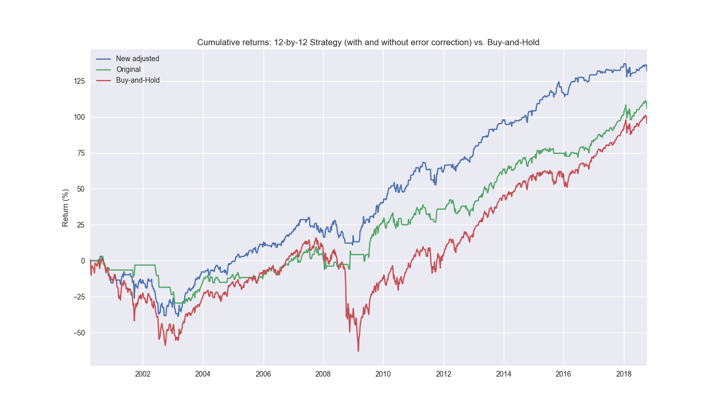
What if we multiplied the error term by the prediction instead? In this case, the directional predictions would skew toward the positive and only on those occasions where the prior prediction was less than the actual would the sign flip.² Doing that produces the following cumulative return chart.

In this case, the new adjusted strategy performs significantly better! It outperforms buy-and-hold and the original strategy by 36% and 26% points, respectively. It enjoys almost twice the cumulative return as the unadjusted strategy. Critically, the new adjusted strategy’s Sharpe ratio is almost double that of buy-and-hold at 0.6 and 0.08 points better than the original. If we had implemented short-selling, the strategy would have performed even better.

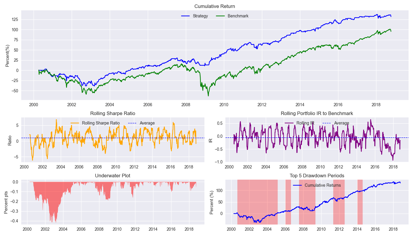
When we plot the various metrics in our handy tearsheet (below) against buy-and-hold, we note that new adjusted strategy suffers similar drawdown periods as the original strategy, but the main advantage appears to be avoiding the really large down moves. Indeed, the new adjusted strategy is out of the market almost 5% more than the original strategy. We’ll present the remaining metrics we’ve used and run the circular block sampling in our next post. After that we come to the pièce de résistance – testing the finished model on out-of-sample data. Stay tuned!

Code below.

# Built using Python 3.10.19 and a virtual environment 

# Load packages
import pandas as pd
import numpy as np
from datetime import datetime, timedelta
import statsmodels.api as sm
import matplotlib.pyplot as plt
from matplotlib.ticker import FuncFormatter
import yfinance as yf
import seaborn as sns
from scipy.stats import ttest_ind

plt.style.use('seaborn-v0_8')
plt.rcParams['figure.figsize'] = (14,8)

def get_spy_weekly_data() -> pd.DataFrame:
    df = yf.download('SPY', start='2000-01-01', end='2024-10-01')
    df.columns = ['open', 'high', 'low', 'close', 'adj close', 'volume']
    df.index.name = 'date'

    # Create training set and downsample to weekly ending Friday
    df_train = df.loc[:'2019-01-01', 'adj close'].copy()
    df_w = pd.DataFrame(df_train.resample('W-FRI').last())
    df_w.columns = ['price'] 

    return df_w

df_w = get_spy_weekly_data()

# Create momentum dictionary
periods = [3, 6, 9, 12]
momo_dict = {}
for back in periods:
    for forward in periods:
        df_out = df_w.copy()
        df_out['ret_back'] = np.log(df_out['price']/df_out['price'].shift(back))
        df_out['ret_for'] = np.log(df_out['price'].shift(-forward)/df_out['price'])
        df_out = df_out.dropna()

        mod = sm.OLS(df_out['ret_for'], sm.add_constant(df_out['ret_back'])).fit()
        momo_dict[f"{back} - {forward}"] = {'data': df_out,
                                            'params': mod.params,
                                            'pvalues': mod.pvalues}


# Trade with error handling
df_trade_1 = momo_dict['12 - 12']['data'].copy()

mod_look_forward = 12
train_pd = 5
test_pd = 1
tot_pd = train_pd + test_pd
lr = 2

trade_pred = []
trade_pred_un = []
trade_pred_old = []
for i in range(tot_pd, len(df_trade_1)-mod_look_forward+1, test_pd):
    train_df = df_trade_1.iloc[i-tot_pd:i-test_pd, 1:]
    valid_df = df_trade_1.iloc[i-test_pd:i, 1:]
    uncorr_df = df_trade_1.iloc[i-test_pd+mod_look_forward-1:i-test_pd+mod_look_forward, 1:]
    test_df = df_trade_1.iloc[i-test_pd+mod_look_forward:i-test_pd+mod_look_forward+1, 1:]

    # Ensure 'ret_back' is 2D by selecting it as a DataFrame, not a Series
    X_train = sm.add_constant(train_df[['ret_back']])
    if valid_df.shape[0] > 1:
        X_valid = sm.add_constant(valid_df[['ret_back']])
    else:
        X_valid = sm.add_constant(valid_df[['ret_back']], has_constant='add')

    if uncorr_df.shape[0] > 1:
        X_uncorr = sm.add_constant(uncorr_df[['ret_back']])
    else:
        X_uncorr = sm.add_constant(uncorr_df[['ret_back']], has_constant='add')

    if test_df.shape[0] > 1:
        X_test = sm.add_constant(test_df[['ret_back']])
    else:
        X_test = sm.add_constant(test_df[['ret_back']], has_constant='add')

    # Fit the model
    mod = sm.OLS(train_df['ret_for'], X_train).fit()

    # Predict using the test data
    pred = mod.predict(X_valid).values
    actual = valid_df['ret_for'].values
    gamma = -(actual - pred)*lr
    pred_old = mod.predict(X_uncorr)
    trade_pred_old.extend(pred_old)

    mod_pred = mod.predict(X_test).values
    trade_pred_un.extend(mod_pred)
    trade_pred.extend(mod_pred * gamma)

assert len(trade_pred) + mod_look_forward + train_pd == len(df_trade_1)
assert len(trade_pred_un) + mod_look_forward + train_pd == len(df_trade_1)

df_trade_1['pred'] = np.concatenate((np.zeros(mod_look_forward + train_pd), np.array(trade_pred)))
df_trade_1['pred_un'] = np.concatenate((np.zeros(mod_look_forward + train_pd), np.array(trade_pred_un)))
df_trade_1['pred_old'] = np.concatenate((np.zeros(mod_look_forward + train_pd - 1), np.array(trade_pred_old), np.zeros(1)))
df_trade_1['ret'] = np.log(df_trade_1['price']/df_trade_1['price'].shift(1))

df_trade_1['signal'] = np.where(df_trade_1['pred'] > 0, 1, 0)
df_trade_1['signal_un'] = np.where(df_trade_1['pred_un'] > 0, 1, 0)
df_trade_1['signal_old'] = np.where(df_trade_1['pred_old'] > 0, 1, 0)
df_trade_1['signal_sh'] = np.where(df_trade_1['pred'] >= 0, 1, -1)

df_trade_1['strat_ret'] = df_trade_1['signal'].shift(1) * df_trade_1['ret']
df_trade_1['strat_ret_un'] = df_trade_1['signal_un'].shift(1) * df_trade_1['ret']
df_trade_1['strat_ret_old'] = df_trade_1['signal_old'].shift(1) * df_trade_1['ret']
df_trade_1['strat_ret_sh'] = df_trade_1['signal_sh'].shift(1) * df_trade_1['ret']

# Plot returns
(df_trade_1[['strat_ret', 'strat_ret_old', 'ret']].cumsum()*100).plot()
plt.ylabel("Return (%)")
plt.xlabel("")
plt.legend(['Corrected', 'Original', 'Buy-and-Hold'])
plt.title('Cumulative returns: 12-by-12 Strategy (with and without error correction) vs. Buy-and-Hold')
plt.show()


# Tearsheet
# For plot_tearsheet function
# See https://www.optionstocksmachines.com/post/2024-11-08-day-16-comps/
plot_tearsheet(df_trade_1['strat_ret'], df_trade_1['ret'], window=13, period=52, save_figure=False, title=None)