Day 29: Out of sample

The moment of truth has arrived! On Day 28, we iterated through all the metrics we had previously used to identify and analyze the robustness of our strategy. We found the new adjusted strategy performed better than the original and adjusted strategies. Such performance was also statistically significant for key scenarios. But on simulation, buy-and-hold beat the new adjusted strategy on average across different sampling methods. Now it’s time to look at how our various strategies would have performed out of sample. Recall, we set up our training to run until the end of 2018. The test period was intended to run from 2019 to end of 2023. A fraught period indeed, but we needed to choose something. Importantly, all of the analyses, modifications, and enhancements were only conducted on the training period in proper data science fashion. We didn’t want any intentional (or unintentional) snooping to occur. Ideally, one should only look once at performance in the test period; otherwise, the test period becomes a shadow training period that might be risky to your wealth.¹ Let’s see how the strategies perform!

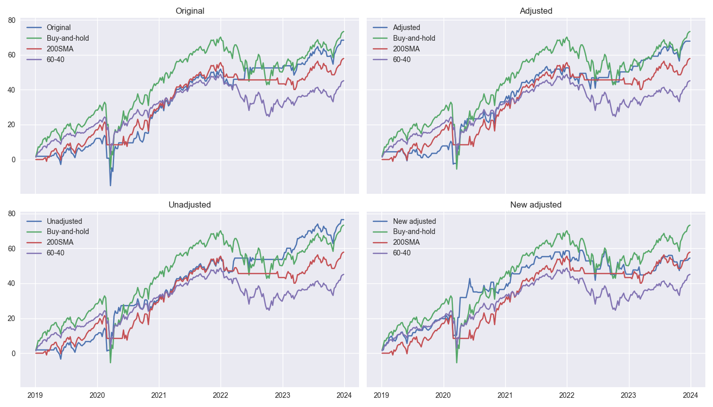
Below, we show the four strategies – original, adjusted, unadjusted, and new adjusted – against the three benchmarks – buy-and-hold, 200-day simple moving average (200SMA), and the SPY-IEF 60%-40% rebalanced (60-40).

Seems like we need some parmesan to go with this spaghetti. Looking at the green line, one notes that buy-and-hold tends to dominate the strategies and the other benchmarks. Both the 200SMA and 60-40 underperform buy-and-hold and the strategies. This is not surprising in the case of the 60-40, given the rise in rates over the 2022-2023 time period. What is surprising is the weakness in the 200SMA. The Hello World of trading strategies just isn’t what it used to be.

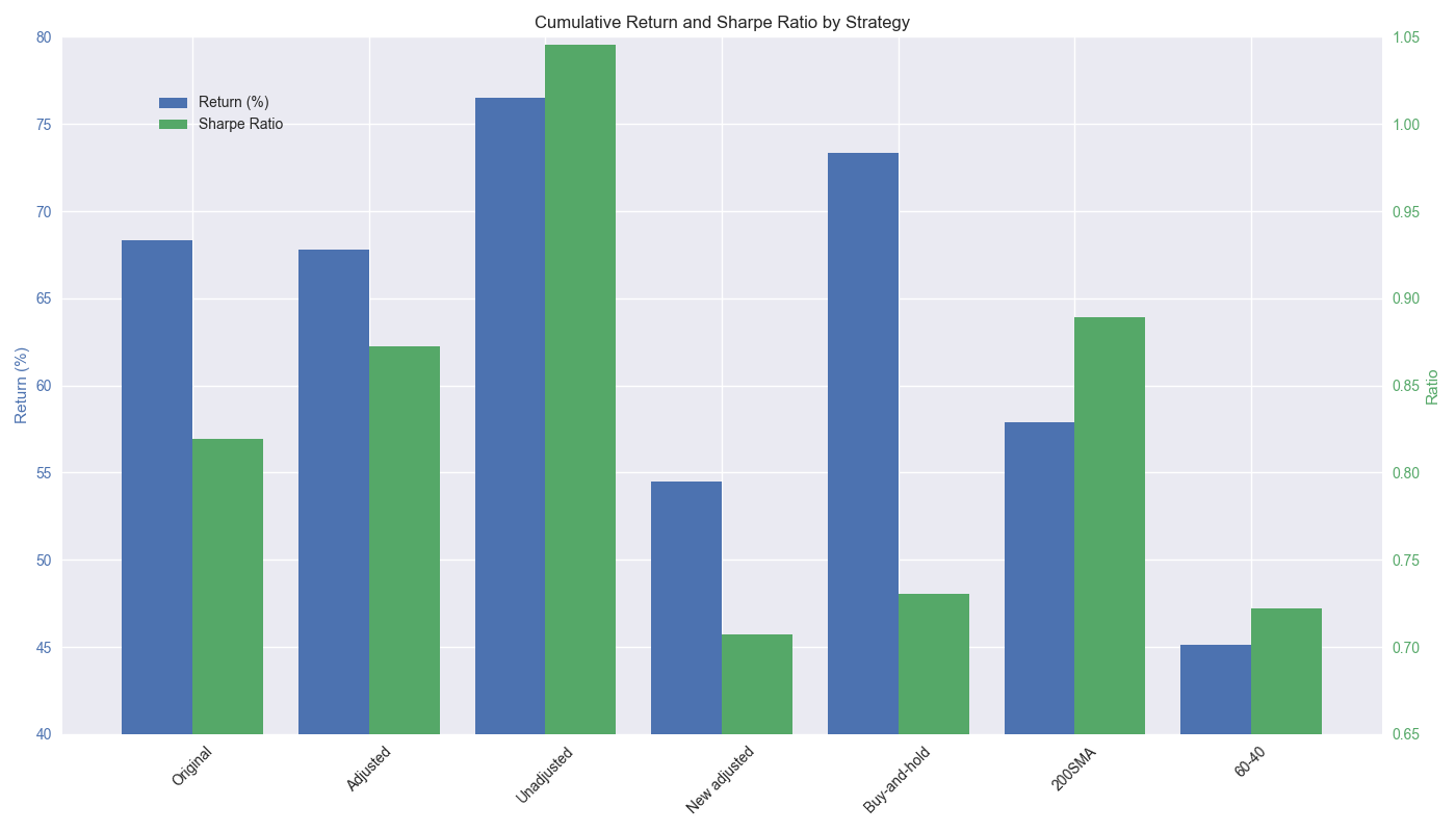
Whatever the case, another surprise is how the unadjusted strategy performed. This was never supposed to be a viable strategy. Indeed, we showed how poorly it did in our training period more as a comparison and to understand why the adjusted strategy performed so well. Yet, out of sample, it beats buy-and-hold! Let’s drill down into cumulative and risk-adjusted returns. We show both for all strategies below.

The cumulative return is shown on the left y-axis and the Sharpe Ratio on the right. We see that original and adjusted strategies perform similarly, with the adjusted edging out the original on the Sharpe Ratio. The unadjusted strategy dominates all others with a Sharpe Ratio greater than 1! That is, extremely rare for such a straightforward strategy and is likely due to the luck of the period. The 60-40 performs the worst during this period. Recall, all those pundit claiming that “60-40 is dead!” in the 2022-2023 timeframe. This is why. The new adjusted strategy is only moderately better than 60-40. Interestingly, even though the 200SMA underperforms on a cumulative return basis, it’s Sharpe outperforms buy-and-hold as well as the original and adjusted strategies. Maybe it was too soon to say goodbye to Hello World!

Given these results and the previous 28 days of backtesting, what should we conclude? First off, it shouldn’t come as a surprise that most of the strategies underperformed buy-and-hold out of sample. A similar phenomenon typically occurs in machine learning, where the error rate usually increases in the test set relative to the training set.² So we should certainly expect performance to slip for the strategies on the test set. That the strategies flipped from out- to underperformance on cumulative returns might seem unacceptable. It certainly doesn’t tell a nice, simple story for prospective investors!

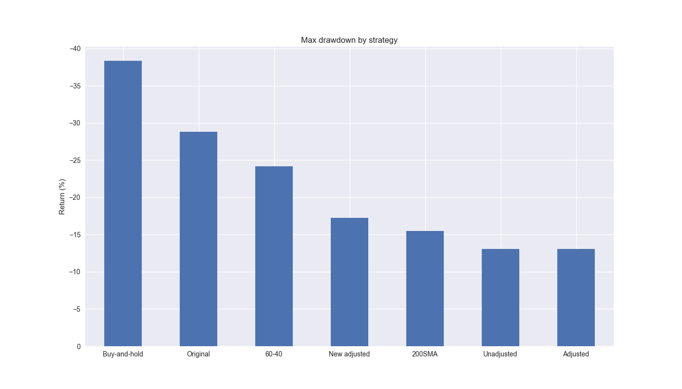
But if the question is, whether to invest in the strategy vs. buy-and-hold, we shouldn’t rely only on cumulative return, which can be path dependent; risk-adjusted returns should take precedence. Indeed, the original and adjusted strategies outperform buy-and-hold by 8-11 points on the Sharpe ratio. On this account, such strategies could be attractive. Additionally, if one is worried about drawdowns, it might be wise to favor the adjusted strategy, which features the lowest drawdown, as shown in the graph below.

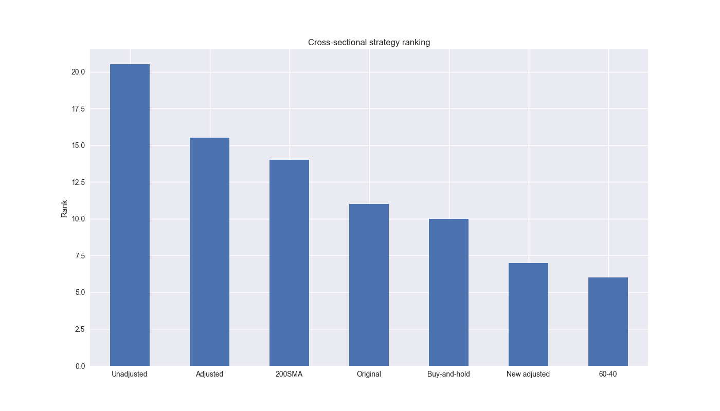
If we rank all the strategies and benchmarks cross-sectionally, the unadjusted strategy dominates, as shown in the plot below. But we would have rejected this strategy in reality due to its underperformance for most of the training period. The adjusted strategy is next, followed by the 200SMA.

Of course, there is still the issue of the original the strategy underperforming buy-and-hold in simulation. We used simulation as an example of a way to quantify the likelihood of outperformance. But the approach was more illustrative than exhaustive. If simulation were to have veto power, we’d want to have conducted more tests and added a degree more sophistication.

Would we employ the adjusted strategy ourselves? We believe that it is an interesting strategy for one that is relatively straightforward. And what we really like about it is that it is relatively easy to explain and has a solid thesis behind it. Could it be refined further? Absolutely! But before that, and from a practical standpoint, we’d need to conduct trade analysis to understand the tax drag better and where the strategy could fit in our overall asset allocation process. But those discussions will have to wait for another series! In our next and final post of the series, we sum up lessons learned and next steps. Stay tuned!

Code below.

# Built using Python 3.10.19 and a virtual environment 


# Load packages
import pandas as pd
import numpy as np
from datetime import datetime, timedelta
import statsmodels.api as sm
import matplotlib.pyplot as plt
from matplotlib.ticker import FuncFormatter
import yfinance as yf

plt.style.use('seaborn-v0_8')
plt.rcParams['figure.figsize'] = (14,8)

def get_spy_weekly_data() -> pd.DataFrame:
    df = yf.download('SPY', start='2000-01-01', end='2024-10-01')
    df.columns = ['open', 'high', 'low', 'close', 'adj close', 'volume']
    df.index.name = 'date'

    # Create training set and downsample to weekly ending Friday
    df_w = df.loc[:,'adj close'].copy()
    df_w = pd.DataFrame(df_w.resample('W-FRI').last())
    df_w.columns = ['price'] 

    return df_w

df_w = get_spy_weekly_data()

# Create momentum dictionary
forward = 12
back = 12
df_out = df_w.copy()
df_out['ret_back'] = np.log(df_out['price']/df_out['price'].shift(back))
df_out['ret_for'] = np.log(df_out['price'].shift(-forward)/df_out['price'])
df_out = df_out.dropna()

# create train and test set
df_train = df_out.loc[:"2019-01-01"]
df_test = df_out.loc["2018-01-01":]
df_train.tail(6)
df_test.head()

# create function to perform walk-forward models
def get_walk_forward(dataf, mod_look_forward, train_pd, test_pd, lr, error_add=True):
        
        tot_pd = train_pd + test_pd
        
        trade_pred = []
        trade_pred_un = []
        trade_pred_old = []
        mod_params = []
        data_out = dataf.copy()

        for i in range(tot_pd, len(dataf)-mod_look_forward+1, test_pd):
            train_df = dataf.iloc[i-tot_pd:i-test_pd, 1:]
            valid_df = dataf.iloc[i-test_pd:i, 1:]
            uncorr_df = dataf.iloc[i-test_pd+mod_look_forward-1:i-test_pd+mod_look_forward, 1:]
            test_df = dataf.iloc[i-test_pd+mod_look_forward:i-test_pd+mod_look_forward+1, 1:]

            # Ensure 'ret_back' is 2D by selecting it as a DataFrame, not a Series
            X_train = sm.add_constant(train_df[['ret_back']])
            if valid_df.shape[0] > 1:
                X_valid = sm.add_constant(valid_df[['ret_back']])
            else:
                X_valid = sm.add_constant(valid_df[['ret_back']], has_constant='add')

            if uncorr_df.shape[0] > 1:
                X_uncorr = sm.add_constant(uncorr_df[['ret_back']])
            else:
                X_uncorr = sm.add_constant(uncorr_df[['ret_back']], has_constant='add')

            if test_df.shape[0] > 1:
                X_test = sm.add_constant(test_df[['ret_back']])
            else:
                X_test = sm.add_constant(test_df[['ret_back']], has_constant='add')

            # Fit the model
            mod = sm.OLS(train_df['ret_for'], X_train).fit()
            mod_params.append(mod.params.values)

            # Predict using the test data
            pred = mod.predict(X_valid).values
            actual = valid_df['ret_for'].values
            
            gamma = -(actual - pred)*lr
            pred_old = mod.predict(X_uncorr)
            trade_pred_old.extend(pred_old)

            mod_pred = mod.predict(X_test).values
            trade_pred_un.extend(mod_pred)
            
            if error_add:
                trade_pred.extend(mod_pred + gamma)
            else:
                trade_pred.extend(mod_pred * gamma)

        assert len(trade_pred) + mod_look_forward + train_pd == len(dataf)
        assert len(trade_pred_un) + mod_look_forward + train_pd == len(dataf)

        data_out['pred'] = np.concatenate((np.zeros(mod_look_forward + train_pd), np.array(trade_pred)))
        data_out['pred_un'] = np.concatenate((np.zeros(mod_look_forward + train_pd), np.array(trade_pred_un)))
        data_out['pred_old'] = np.concatenate((np.zeros(mod_look_forward + train_pd - 1), np.array(trade_pred_old), np.zeros(1)))
        data_out['ret'] = np.log(data_out['price']/data_out['price'].shift(1))

        data_out['signal'] = np.where(data_out['pred'] > 0, 1, 0)
        data_out['signal_un'] = np.where(data_out['pred_un'] > 0, 1, 0)
        data_out['signal_old'] = np.where(data_out['pred_old'] > 0, 1, 0)
        data_out['signal_sh'] = np.where(data_out['pred'] >= 0, 1, -1)

        data_out['strat_ret'] = data_out['signal'].shift(1) * data_out['ret']
        data_out['strat_ret_un'] = data_out['signal_un'].shift(1) * data_out['ret']
        data_out['strat_ret_old'] = data_out['signal_old'].shift(1) * data_out['ret']
        data_out['strat_ret_sh'] = data_out['signal_sh'].shift(1) * data_out['ret']

        return data_out

# Set parameters
mod_look_forward = 12
train_pd = 5
test_pd = 1
lr = 2

# Run strategies        
df_trade_train_add = get_walk_forward(df_train, mod_look_forward=mod_look_forward, train_pd=train_pd, test_pd=test_pd, lr=lr)
df_trade_train_mul = get_walk_forward(df_train, mod_look_forward=mod_look_forward, train_pd=train_pd, test_pd=test_pd, lr=lr, error_add=False)

df_trade_test_add = get_walk_forward(df_test, mod_look_forward=mod_look_forward, train_pd=train_pd, test_pd=test_pd, lr=lr)
df_trade_test_mul = get_walk_forward(df_test, mod_look_forward=mod_look_forward, train_pd=train_pd, test_pd=test_pd, lr=lr, error_add=False)


# Load data for other strategies
# 60-40
df = pd.read_csv('data/spy_ief_close.csv', parse_dates=['date'], index_col='date')
df_bw =  pd.DataFrame(df.resample('W-FRI').last())
df_bw[['ief_chg', 'spy_chg']] = df_bw[['ief','spy']].apply(lambda x: np.log(x/x.shift(1)))

start_date = '2019-01-01'
end_date = "2024-01-01"

bench_returns = df_bw[['ief_chg', 'spy_chg']].copy()
bench_returns = bench_returns.loc[start_date:end_date]

weights = [0.4,0.6]
bench_60_40_rebal = calculate_portfolio_performance(weights, bench_returns, rebalance=True, frequency='quarter')
bench_60_40_rebal.index = bench_60_40_rebal.index.tz_localize(None) #type:ignore

# 200-day SMA
df_200 = df_w.copy()
df_200.columns = ['price']
df_200 = df_200.resample('W-FRI').last()
# 40 weeks = 200 days
df_200['sma_200'] = df_200['price'].rolling(40).mean()
df_200['ret'] = np.log(df_200['price']/df_200['price'].shift(1))
df_200['signal'] = np.where(df_200['price'] > df_200['sma_200'], 1, 0)
df_200['strat_ret'] = df_200['signal'].shift(1)*df_200['ret']

df_200_bench = df_200.loc[start_date:end_date]
df_200_bench['strat_ret'], window=13, period=52, save_figure=False, title='strat_12-12_60-40')

# Concatenate strategies
df_all = pd.concat([df_trade_test_mul.loc[start_date:end_date, ['strat_ret', 'strat_ret_old', 'strat_ret_un', 'ret']], 
           df_trade_test_add.loc[start_date:end_date, ['strat_ret']], 
           df_200_bench['strat_ret'],
           bench_60_40_rebal],
           axis=1)

df_all.columns = ['New adjusted', 'Original', 'Unadjusted', 'Buy-and-hold', 'Adjusted', '200SMA', '60-40']

strategies = ['Original', 'Adjusted', 'Unadjusted', 'New adjusted']
benchmarks = ['Buy-and-hold','200SMA', '60-40']

# Plot all strategies cumulative performance
fig, axes = plt.subplots(2,2,sharex=True, sharey=True)

for idx, ax in enumerate(fig.axes):
    ax.plot(df_all.index, (df_all[[strategies[idx]] + benchmarks].cumsum()*100).values)
    ax.legend([strategies[idx]] + benchmarks)
    ax.set_title(strategies[idx])

plt.tight_layout()
plt.show()

# Data preparation
cumulative_returns = (df_all[strategies + benchmarks].cumsum().iloc[-1] * 100)
sharpe_ratios = df_all[strategies + benchmarks].apply(sharpe)

# Define the positions of the bars
x = np.arange(len(cumulative_returns))  # Bar positions
width = 0.4  # Width of each bar

# Seaborn defaults for colors
blue_sns = '#4C72B0'
green_sns = '#55A868'

# Create the figure and the first y-axis
fig, ax1 = plt.subplots()

# Plot the cumulative returns
bars1 = ax1.bar(x - width/2, cumulative_returns, width, color=blue_sns, label='Return (%)')
ax1.set_ylabel('Return (%)', color=blue_sns)
ax1.tick_params(axis='y', labelcolor=blue_sns)
ax1.set_ylim(40, 80)  # Adjust as needed

# Add the second y-axis for Sharpe ratios
ax2 = ax1.twinx()
bars2 = ax2.bar(x + width/2, sharpe_ratios, width, color=green_sns, label='Sharpe Ratio')
ax2.set_ylabel('Ratio', color=green_sns)
ax2.tick_params(axis='y', labelcolor=green_sns)
ax2.set_ylim(0.65, 1.05)  # Adjust as needed

# Add the x-axis labels
ax1.set_xticks(x)
ax1.set_xticklabels(cumulative_returns.index, rotation=45)
ax2.grid(False)

# Add a title
plt.title('Cumulative Return and Sharpe Ratio by Strategy')

# Add a legend
fig.legend(loc='upper left', bbox_to_anchor=(0.1, 0.9))

# Show the plot
plt.tight_layout()
plt.show()


# Create drawdown dictionay
drawdown_dict = {}
for strat in df_all.columns:
    drawdown, top_dd_periods = plot_drawdowns(df_all[strat].cumsum())
    drawdown_dict[strat] = {'drawdown': drawdown,
                            'top_dd_periods': top_dd_periods}

# Create drawdown dataframe
df_dd = pd.DataFrame(columns=['drawdown'], index=df_all.columns)
for strat in df_all.columns:
    df_dd.loc[strat, 'drawdown'] = drawdown_dict[strat]['drawdown'].min()

# Plot drawdowns
ax = (df_dd.sort_values("drawdown", ascending=True)*100).plot(kind='bar', rot=0)
ax.set_ylabel('Return (%)')
ax.invert_yaxis()
ax.legend('')
ax.set_title('Max drawdown by strategy')
plt.show()

# create rank dataframe and plot
(pd.concat([cumulative_returns, sharpe_ratios, df_dd], axis=1)
.rank(axis=0)
.sum(axis=1)
.sort_values(ascending=False)).plot(kind='bar', rot=0)
plt.ylabel('Rank')
plt.title('Cross-sectional strategy ranking')
plt.show()