Rebalancing ruminations
Back in the rebalancing saddle! In our last post on rebalancing, we analyzed whether rebalancing over different periods would have any effect on mean or risk-adjusted returns for our three (equal, naive, and risky) portfolios. We found little evidence that returns were much different whether we rebalanced monthly, quarterly, yearly, or not at all. Critically, as an astute reader pointed out, if these had been taxable accounts, the rebalancing would likely have been a drag on performance. This is clearly an important point that we will address in later posts.
Even though our tests suggested rebalancing wasn’t worth the effort, we decided to proceed. In truth, while our three ETF portfolios were meant to approximate the major asset classes, they didn’t mimic the benchmark portfolio we constructed all that well. However, that portfolio suffered from limited data. So we simulated a 10-year period for a portfolio whose components matched the historical return and risk profiles of the major asset classes. Here again we found little evidence that rebalancing did much.
But this lack of evidence, doesn’t mean there’s evidence of a lack of better returns from rebalancing. We believe a broader test is required. To that end, we’ll run many simulations of those historical returns to identify the likelihood that rebalancing is worthwhile. Recall that since we’ve been using historical data, we’re really only looking at one observation because historical events are necessarily independent of one another. If Caesar hadn’t crossed the Rubicon, the French Revolution might never have happened! The best way to test rebalancing would be to aggregate data from a thousand alternate realities. Sadly access to such data only shows up in science fiction. We’ll have to make do with the next best thing: the power of R programming. Strap in, we’re headed down the wormhole of simulations!
As before, we’ll run a simulation using the historical mean and standard deviation of return for US and non-US stocks and bonds as well as the S&P GSCI Commodity Total Return index. But this time we’ll run a 1,000 of those simulations and then aggregate them.1 Additionally, we’ll equal weight the assets as a starting point. Our first test will be to see how often the mean return of one rebalancing strategy exceeds that of another.
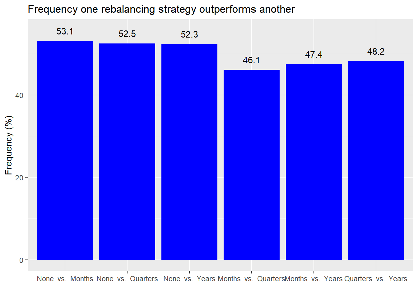
Not exactly a resounding result. But we see that no rebalancing tends to outperform other rebalancing strategies a little bit better than a coin flip. Comparing rebalancing strategies against one another shows that rebalancing more frequently tends to underperform rebalancing less frequently. But here it’s only slightly less than coin flip too.
Let’s look at the mean returns and range of outcomes to get a sense of the overall performance.
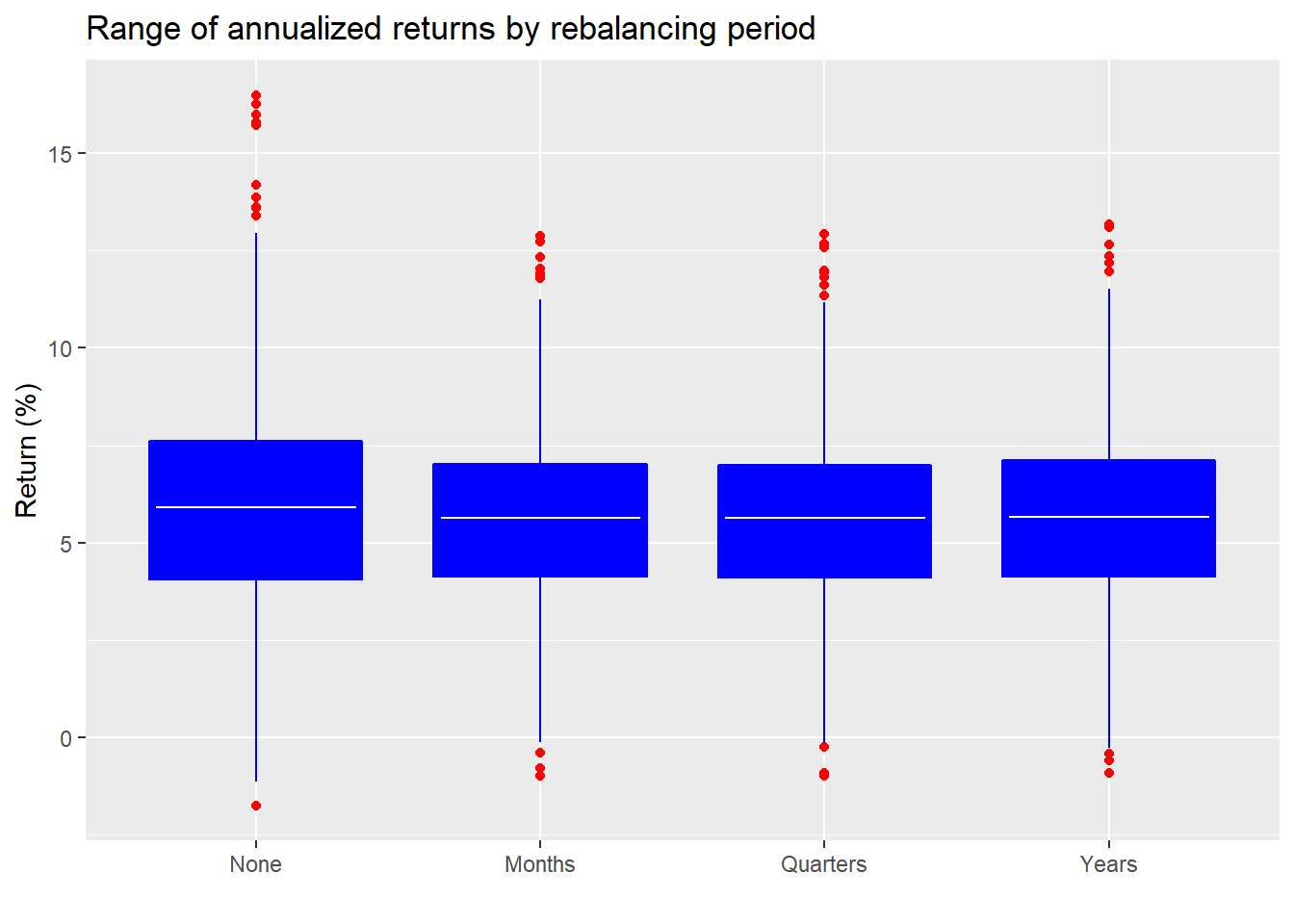
The white horizontal lines represent the average of all the simulations’ annualized returns. The bottom and top edge of the boxes represent the middle 50% of all observations. There doesn’t seem to be much of difference, though it’s clear that no rebalancing results in a wider range of outcomes. Eyeballing this suggests that there really shouldn’t be much of a difference in the mean return. However, to check the significance we need to be careful how we run the test. If we test the mean returns from no rebalancing for all simulations against the other rebalancing periods we’ll be comparing results from different simulations. This is different from comparing returns within each simulation using t-tests and then calculating mean p-value from all the simulations. The latter seems more accurate.2
| Comparison | P-value |
|---|---|
| None vs. Months | 0.84 |
| None vs. Quarters | 0.84 |
| None vs. Years | 0.85 |
| Months vs. Quarters | 0.98 |
| Months vs. Years | 0.95 |
| Quarters vs. Years | 0.96 |
Another strike against rebalancing. We see that on average, the p-values are quite high, suggesting any difference in mean returns is likely due to chance. Now let’s check risk-adjusted returns using the Sharpe ratio.
| Period | Ratio |
|---|---|
| None | 0.72 |
| Months | 0.76 |
| Quarters | 0.76 |
| Years | 0.76 |
No rebalancing produces a slightly worse risk-adjusted return than rebalancing. But is the difference significant? Our guess is probably not. Performing a robust test would require some more complicated math that would be beyond the scope of this post to explain. Instead, we’ll look at the number of occurrences in which one rebalancing regime produced a better Sharpe ratio than another. The assumption is that if it’s greater than 90%, the differences are probably significant.
| Periods | Occurence |
|---|---|
| None vs. Months | 24.7 |
| None vs. Quarters | 24.4 |
| None vs. Years | 25.6 |
| Months vs. Quarters | 51.0 |
| Months vs. Years | 56.6 |
| Quarters vs. Years | 56.5 |
As the table shows even though rebalancing did produce better Sharpe ratios than no rebalancing a majority of the time, it didn’t do so more than 90% of the time.
Is this the end of our analysis? No because we looked at an equal-weighted portfolio. Perhaps a different weighting scheme would produce different relative results. The prior weighting scheme effectively had a 40% weighting to both stocks and bonds, and a 20% weighting to commodities. Our new weighting scheme will have a 60% weighting to stocks, a 35% weighting to bonds, and a 5% weighting to commodities. This is close to the empirical recommendation of a 60/40 stock/bond portfolio many financial advisors recommend. We’ll run 1,000 simulations and output the same analyses as above.
First, the frequency of outperformance.
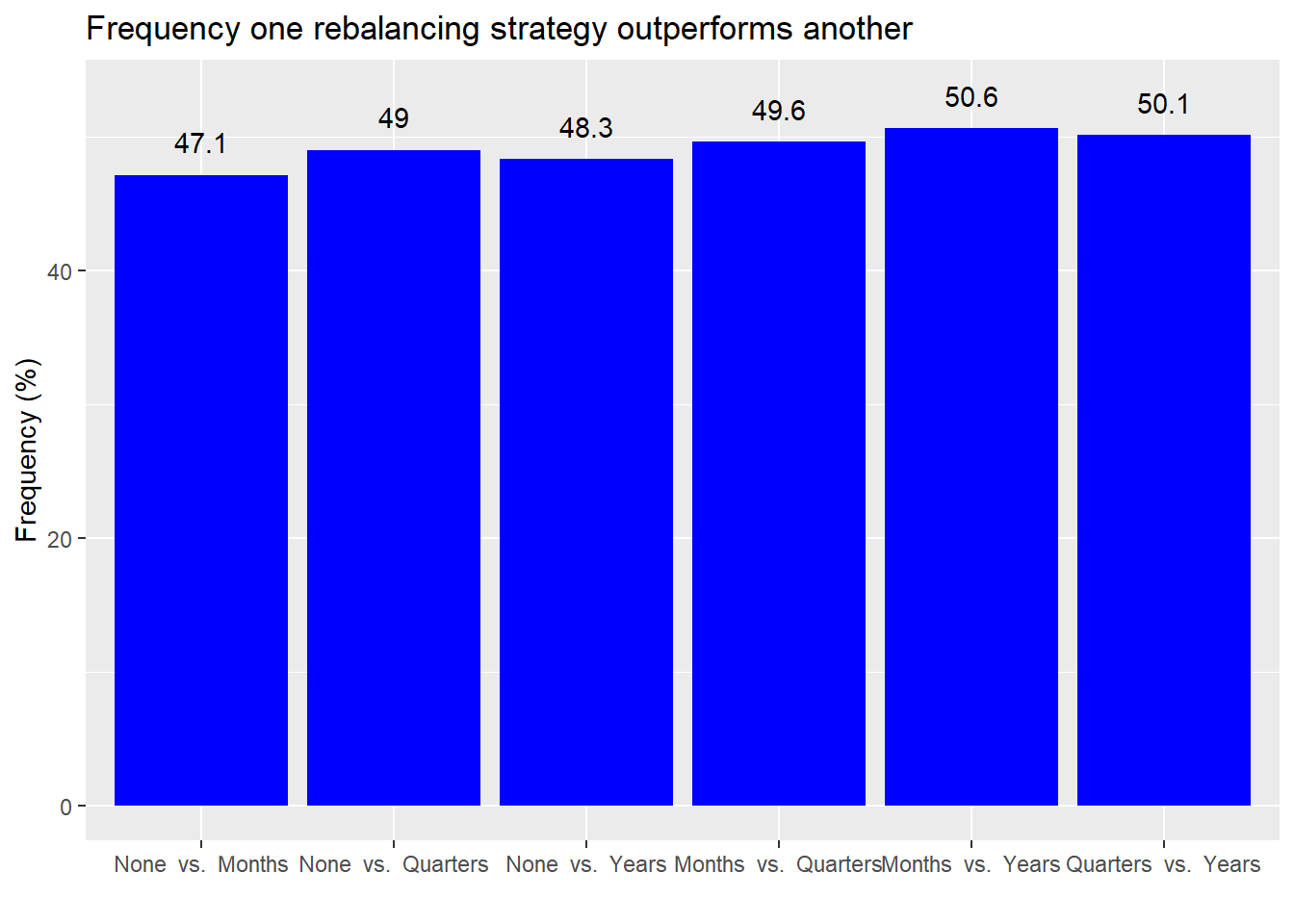
On a different weighting scheme, rebalancing appears to outperform not rebalancing, but only slightly better than a coin toss. Interestingly, there appears to be almost no difference in performance among different rebalancing periods. Are these results significant?
| Comparison | P-value |
|---|---|
| None vs. Months | 0.87 |
| None vs. Quarters | 0.87 |
| None vs. Years | 0.88 |
| Months vs. Quarters | 0.98 |
| Months vs. Years | 0.96 |
| Quarters vs. Years | 0.96 |
Again, not much to see here. Even if the occurrence is somewhat better than 50/50, the differences aren’t significant. We’ll move along to at the Sharpe ratio for the different strategies.
| Period | Ratio |
|---|---|
| None | 0.63 |
| Months | 0.67 |
| Quarters | 0.67 |
| Years | 0.66 |
Like the previous simulation, no rebalancing returned a Sharpe ratio that was 30-40bps lower than the rebalancing strategies. To see if that’s significant we calculate the frequency in which one strategy had a better Sharpe ratio than another.
| Periods | Occurence |
|---|---|
| None vs. Months | 23.3 |
| None vs. Quarters | 23.7 |
| None vs. Years | 26.2 |
| Months vs. Quarters | 53.8 |
| Months vs. Years | 60.7 |
| Quarters vs. Years | 59.5 |
Here too the frequency of a better Sharpe ratio was quite similar to the previous weighting scheme. And there was no occurrence better than 90%.
Where does this leave us? Rebalancing does not appear to produce better returns, risk-adjusted or otherwise. Are there problems with this study? Yes. First, we only tested rebalancing based on timing. In our mind, timing alone is a sort of silly reason to rebalance. What difference does it make to deciding whether to rebalance or not whether a month or a year has passed? Rebalancing based on a threshold seems more logical. Of course, one can rebalance at the end of certain periods if a threshold has been crossed to prevent over trading. Thus, we’d need to conduct a different rebalancing simulation based on some threshold.
The second problem with our tests is that our simulations were based on random samples pulled from a normal distribution. Asset returns have been shown to be non-normal; that is, (without getting too deep into stats) they don’t have a nice bell-shaped curve, are often skewed to one side, and have a lot of outliers. That means our simulated results could be much different than what is likely to occur in reality, perhaps significantly.
A third problem has to do with correlations: they change and they’re often serial. On the first issue, correlations change over time. In periods of high positive correlation, there’s probably no reason to rebalance, as the original weighting likely remains stable. But in periods of low correlation, rebalancing should help because when one is selling upwardly trending assets to buy downward ones, and those trends reverse, the rebalanced portfolio theoretically would exploit that trend reversal.
But there’s a nuance. Rebalancing implicitly assumes correlations don’t change much over time. They certainly aren’t supposed to flip signs. Assets that are negatively correlated aren’t supposed to become positive. Yet this happens and might happen right after one rebalances, potentially nullifying the intended purpose of rebalancing.
We did not explicitly simulate different correlation scenarios, as we assumed the randomness of simulating each asset’s return implicitly introduced different correlations. That assumption might not be correct. Do the simulations produce enough diverse correlation scenarios to do justice to rebalancing? To answer that would require an entire post on its own, which will have to wait.
Then there’s serial correlation, or the phenomenon where current period results are related to any number of past periods. This is important because time series data, especially asset returns, exhibit modest to high amounts of serial correlation. If our simulations don’t account for that phenomenon, then we’re not really approximating real data.
Many of these problems can be resolved by sampling from historical data. Since historical data is non-normal, skewed, and features more outliers, then that would be expressed in the simulations. The same goes for changing and serial correlations, though adjusting for that requires a bit more art.3
Clearly there’s a lot more wood to chop to figure out if rebalancing produces better risk-adjusted returns given the issues we’ve highlighted. From a reproducibility standpoint, it’s tough to find the last 50 years of global stock and bond returns from a freely available source. A bigger question is whether the effort is worth it. If rebalancing really were a source of better returns, wouldn’t it be obvious even from a somewhat flawed simulation? We’d love to know what our readers think. Want more on rebalancing or is it time to move on? Please send us a message at the email after the code with your view.
For those interested in reading more about rebalancing, we’ve included a (hopefully!) balanced representation of the argument in the links below.
Links:
Until next time, here’s the code behind our analyses.
# Load packages
library(tidyquant)
library(tidyverse)

## Create rebalancing simulation function
rebal_sim <- function(wt,...){
  stock_us <- rnorm(120, 0.08/12, 0.2/sqrt(12))
  stock_world <- rnorm(120, 0.065/12, 0.17/sqrt(12))
  bond_us <- rnorm(120, 0.024/12, 0.1/sqrt(12))
  bond_world <- rnorm(120, 0.025/12, 0.14/sqrt(12))
  commod <- rnorm(120, 0.007, 0.057)

  if(missing(wt)){
    wt <- rep(.2, 5)
  }else{
    wt <- wt
  }

  date <- seq(as.Date("2010-02-01"), length = 120, by = "months")-1
  port <- as.xts(cbind(stock_us, stock_world, bond_us, bond_world, commod),
                 order.by = date)

  port_list <- list()
  rebals = c("none","months", "quarters", "years")

  for(pd in rebals){
    if(pd == "none"){
      port_list[[pd]] <- Return.portfolio(port, wt)
    }else{
      port_list[[pd]] <- Return.portfolio(port, wt, rebalance_on = pd)
    }
  }

  port_r <- port_list %>%
    bind_cols() %>%
    data.frame() %>%
    mutate_all(as.numeric) %>%
    mutate(date = date) %>%
    select(date, everything())

  corr <- cor(cbind(stock_us, stock_world, bond_us, bond_world, commod))

  results <- list(port_r = port_r, corr = corr)

  results
}

## Rum simulation

set.seed(123)
rebal_test <- list()
for(i in 1:1000){
  rebal_test[[i]] <- rebal_sim()
}

## Find percentage of time one rebalancing period generates higher returns than another
# Create means comparison function
freq_comp <- function(df){
  count <- 1
  opf <- data.frame(comp = rep(0,6), prob = rep(0,6))
  port_names <-  c("None", "Months", "Quarters", "Years")

  for(i in 1:4){
    for(j in 2:4){
      if(i < j & count < 7){
        opf[count,1] <- paste(port_names[i], " vs. ", port_names[j])
        opf[count,2] <- mean(df[,i]) > mean(df[,j])
        count <- count + 1
      }
    }
  }
  opf
}

# Aggregate function across simulations
prop_df <- matrix(rep(0,6000), nrow = 1000)
for(i in 1:1000){
  prop_df[i,] <- freq_comp(rebal_test[[i]][,2:5])[,2]
}

short_names <-  c("n", "m", "q", "y")
df_names <- c()
count <- 1
for(i in 1:4){
  for(j in 2:4){
    if(i < j & count < 7){
      df_names[count] <- paste(short_names[i], " vs. ", short_names[j])
      count <- count+1
    }
  }
}

rebal_names <- c("None", "Months", "Quarters", "Years")
long_names <- c()
count <- 1
for(i in 1:4){
  for(j in 2:4){
    if(i < j & count < 7){
      long_names[count] <- paste(rebal_names[i], " vs. ", rebal_names[j])
      count <- count + 1
    }
  }
}

prop_df <- prop_df %>% data.frame %>%
  `colnames<-`(df_names)

prop_df %>%
  summarize_all(mean) %>%
  `colnames<-`(long_names) %>%
  gather(key, value) %>%
  mutate(key = factor(key, levels = long_names)) %>%
  ggplot(aes(key,value*100)) +
  geom_bar(stat = "identity", fill = "blue")+
  labs(x= "",
       y = "Frequency (%)",
       title = "Number of times one rebalancing strategy outperforms another") +
  geom_text(aes(label = value*100), nudge_y = 2.5)


## Average results
rebal_mean_df <- data.frame(none = rep(0,1000),
                            monthly = rep(0,1000),
                            quarterly = rep(0,1000),
                            yearly = rep(0,1000))
for(i in 1:1000){
  rebal_mean_df[i,] <- colMeans(rebal_test[[i]][,2:5]) %>% as.vector()
}

# Boxplot of reults
rebal_mean_df %>%
  `colnames<-`(port_names) %>%
  gather(key,value) %>%
  mutate(key = factor(key, levels = port_names)) %>%
  ggplot(aes(key,value*1200)) +
  geom_boxplot(fill = "blue", color = "blue", outlier.colour = "red") +
  stat_summary(geom = "crossbar", width=0.7, fatten=0, color="white",
               fun.data = function(x){ return(c(y=mean(x), ymin=mean(x), ymax=mean(x))) })+
  labs(x = "",
       y = "Return (%)",
       title = "Range of mean annualized returns by rebalancing period")

# Create function
t_test_func <- function(df){
  count <-  1
  t_tests <- c()

  for(i in 1:4){
    for(j in 2:4){
      if(i < j & count < 7){
        t_tests[count] <- t.test(df[,i],df[,j])$p.value
        count <- count +1
      }
    }
  }

  t_tests
}

t_test_func(rebal_test[[995]][,2:5])

t_tests <- matrix(rep(0,6000), ncol = 6)
for(i in 1:1000){
  t_tests[i,] <- t_test_func(rebal_test[[i]][,2:5])
}

t_tests <- t_tests %>%
  data.frame() %>%
  `colnames<-`(long_names)

t_tests %>%
  summarise_all(function(x) round(mean(x),2)) %>%
  gather(Comparison, `P-value`) %>%
  knitr::kable(caption = "Aggregate p-values for simulation")


## Sharpe ratios
sharpe <- matrix(rep(0,4000), ncol = 4)
for(i in 1:1000){
  sharpe[i,] <- apply(rebal_test[[i]][,2:5], 2, mean)/apply(rebal_test[[i]][,2:5],2, sd) * sqrt(12)
}

sharpe <- sharpe %>%
  data.frame() %>%
  `colnames<-`(port_names)

# Table
sharpe %>%
  summarise_all(mean) %>%
  gather(Period, Ratio) %>%
  mutate(Ratio = round(Ratio,3)) %>%
  knitr::kable(caption = "Sharpe ratios by rebalancing period")

sharpe_t <- data.frame(Periods = names(t_tests), Occurence = rep(0,6))
count <- 1
for(i in 1:4){
  for(j in 2:4){
    if(i <j & count < 7){
      sharpe_t[count,2] <- mean(sharpe[,i] > sharpe[,j])
      count <- count + 1
    }
  }
}

sharpe_t %>%
  knitr::kable(caption = "Frequency of better Sharpe ratio")

# Load data
wt1 <- (0.3, 0.3, 0.2, 0.15, 0.05)
rebal_wt <- rebal_sim(wt=wt1)

# Aggregate function across simulations
means_wt_df <- matrix(rep(0,6000), nrow = 1000)
for(i in 1:1000){
  means_wt_df[i,] <- means_comp(rebal_wt[[i]][,2:5])[,2]
}

# Graph
means_wt_df %>%
  summarize_all(mean) %>%
  `colnames<-`(long_names) %>%
  gather(key, value) %>%
  mutate(key = factor(key, levels = long_names)) %>%
  ggplot(aes(key,value*100)) +
  geom_bar(stat = "identity", fill = "blue")+
  labs(x= "",
       y = "Frequency (%)",
       title = "Number of times one rebalancing strategy outperforms another") +
  geom_text(aes(label = value*100), nudge_y = 2.5)

## Run t-test
t_tests_wt <- matrix(rep(0,6000), ncol = 6)
for(i in 1:1000){
  t_tests_wt[i,] <- t_test_func(rebal_wt[[i]][,2:5])
}

t_tests_wt <- t_tests_wt %>%
  data.frame() %>%
  `colnames<-`(long_names)

t_tests_wt %>%
  summarise_all(function(x) round(mean(x),2)) %>%
  gather(Comparison, `P-value`) %>%
  knitr::kable(caption = "Aggregate p-values for simulation")

## Sharpe ratios0
sharpe_wt <- matrix(rep(0,4000), ncol = 4)
for(i in 1:1000){
  sharpe_wt[i,] <- apply(rebal_wt[[i]][,2:5], 2, mean)/apply(rebal_wt[[i]][,2:5],2, sd) * sqrt(12)
}

sharpe_wt <- sharpe_wt %>%
  data.frame() %>%
  `colnames<-`(port_names)

# table
sharpe_wt %>%
  summarise_all(mean) %>%
  gather(Period, Ratio) %>%
  mutate(Ratio = round(Ratio,2)) %>%
  knitr::kable(caption = "Sharpe ratios by rebalancing period")

# Permutation test for sharpe
sharpe_wt_t <- data.frame(Periods = names(t_tests_wt), Occurence = rep(0,6))
count <- 1
for(i in 1:4){
  for(j in 2:4){
    if(i <j & count < 7){
      sharpe_wt_t[count,2] <- mean(sharpe_wt[,i] > sharpe_wt[,j])
      count <- count + 1
    }
  }
}

# Table
sharpe_wt_t %>%
  knitr::kable(caption = "Frequency of getting a better Sharpe ratio")
If you try to reproduce the simulation note that it may take a while to run. If anyone has a better idea on how to write better code for this simulation, please send us an email.↩
This method is perhaps not academically correct, but we hope it is sufficient to reveal some insights.↩
Clearly, beyond the scope of this post, but we’d need to sample returns in a block, That is, we’d choose a representative length and then sample blocks of returns based on that length. The length would approximate the highest serial correlation period of that particular asset. But if you’re simulating more than one asset, each with a different order of serial correlation, which lag do you use?↩