Rolling regime
Our last post finished up examining the three different methods used to predict market regimes in the Gold Miners ETF, GDX – namely, clustering, Gaussian Mixture Methods (GMMs), and Hidden Markov Models (HMMs). We found GMMs performed the best in terms of proof-of-concept. But there was a lot of work to do to go from backtest to viable trading strategy.
In the next few posts, we’ll look at some of the ways we can improve our backtests. Critically, we’ll examine more timely updates to regime detection. The prior models used a 20-day lookback to retrain the algorithm, while retaining the same start date. Although this structure might be okay in some circumstances, it also implies that the weight of new information declines with each update. If you have 100 days of data, each day weighs 1%. If you add 20 days, each day weighs 0.83%, and the most recent 20 days weigh about 17% less in the retrained model vs. the prior most recent 20 days did in the prior model.
What to do? Roll forward so the model is retrained periodically on the same window size. Deciding on the appropriate window size and cadence is not trivial. But we won’t focus on that now. Instead, we’ll use the clustering algorithm with a 252-day window (the rough number of trading days in a year) and a retrain trigger every 20 days.
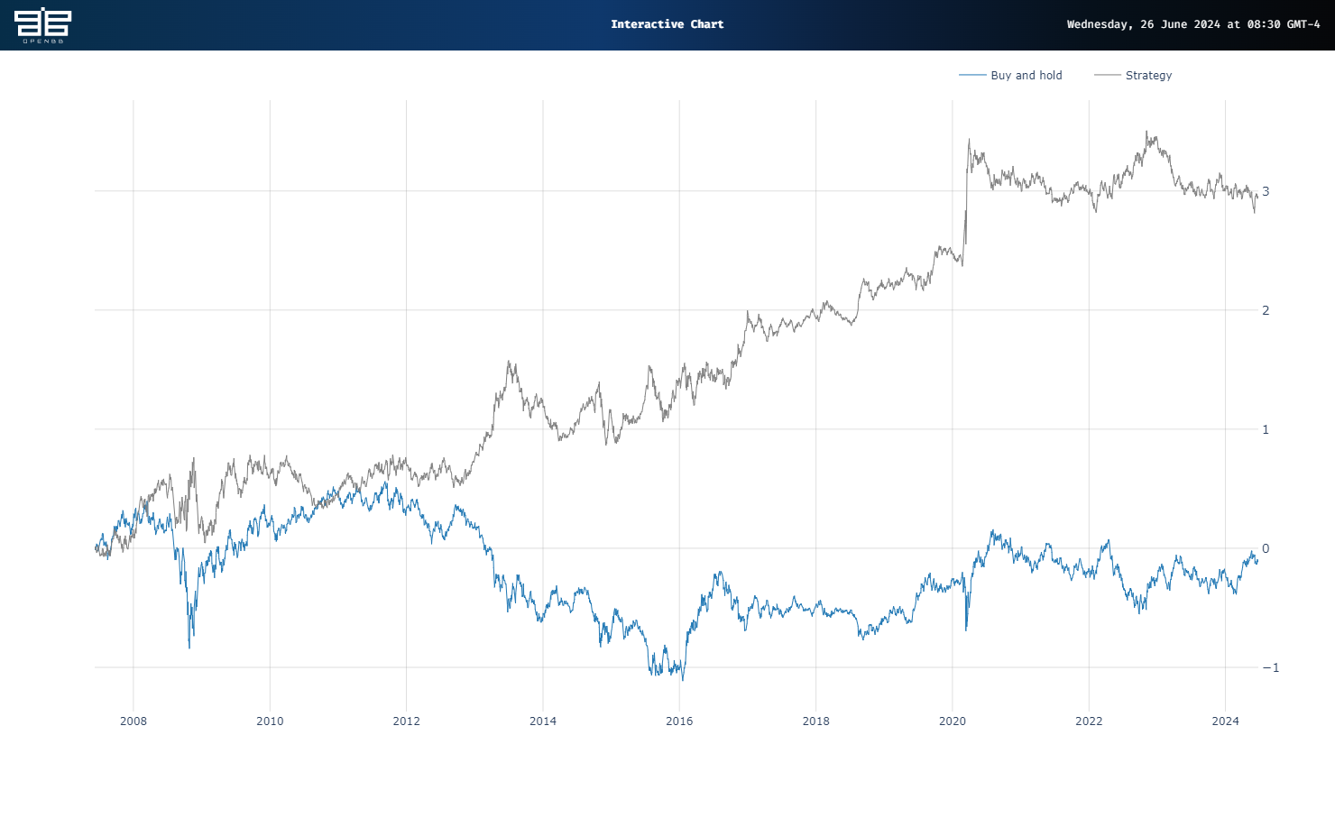
Then, as before, we use the model outputs as signals to buy/sell the ETF. We graph the results below.

The results are dramatic. Almost too good to be true. Buy and hold generates less than a -10% cumulative return while the Strategy produces a 281% cumulative return, or almost 300 points of outperformance! Recall in the previous clustering backtest, the Strategy outperformed by about 20 points in the test period.
However, execution is everything. If we delayed trading on the signal by a day, performance drops precipitously – essentially flat, though it still outperforms relative to Buy and hold. Recall most proof-of-concept backtests are based on end-of-day data and assume you execute at the close of the day the signal is generated.
Executing a day later is unrealistic just as much as executing on the day of. But introducing more realistic execution becomes fraught without intraday data, an obstacle on its own if you want reproducibility.
Whatever the case, shortening the training period and keeping its length stable over the test timeframe appears to yield some intriguing results. Next time will run the same analyses on GMMs and HMMs.
Here’s the code.
# Built using Python 3.10.19 and a virtual environment

# Install packages
from openbb import obb
import numpy as np
import pandas as pd
from hmmlearn.hmm import GaussianHMM
from sklearn.cluster import AgglomerativeClustering
from sklearn.mixture import GaussianMixture
import math
import warnings
warnings.filterwarnings('ignore')
import yfinance as yf
import matplotlib.pyplot as plt

# Functions
def prepare_data_for_model_input(prices: pd.DataFrame, ma: int, instrument: str) -> pd.DataFrame | np.ndarray:
    """
    Returns a dataframe with prices, moving average, and log returns as well as np.array of log returns
    """
    prices[f'{instrument}_ma'] = prices[instrument].rolling(ma).mean()
    prices[f'{instrument}_log_return'] = np.log(prices[f'{instrument}_ma']/prices[f'{instrument}_ma'].shift(1)).dropna()

    prices = prices.dropna()
    prices_array = prices[f'{instrument}_log_return'].values.reshape(-1,1)

    return prices, prices_array

class RegimeDetection:

    """
    Object to hold clustering, Gaussian Mixture or Hidden Markov Models
    """
    def get_regimes_hmm(self, input_data, params):
        hmm_model = self.initialise_model(GaussianHMM(), params).fit(input_data)
        return hmm_model

    def get_regimes_clustering(self, params):
        clustering =  self.initialise_model(AgglomerativeClustering(), params)
        return clustering

    def get_regimes_gmm(self, input_data, params):
        gmm = self.initialise_model(GaussianMixture(), params).fit(input_data)
        return gmm

    def initialise_model(self, model, params):
        for parameter, value in params.items():
            setattr(model, parameter, value)
        return model

def feed_forward_training(model: RegimeDetection, params: dict, prices: np.array, split_index: int, retrain_step: int, cluster: bool = False, roll: bool = False) -> list:
    """
    Returns list of regime states
    """

    # train/test split and initial model training
    init_train_data = prices[:split_index]
    test_data = prices[split_index:]
    if cluster:
        rd_model = model(params)
    else:
        rd_model = model(init_train_data, params)

    # predict the state of the next observation
    states_pred = []
    for i in range(math.ceil(len(test_data))):
        start_index = i if roll else 0

        split_index += 1
        if cluster:
            preds = rd_model.fit_predict(prices[start_index:split_index]).tolist()
        else:
            preds = rd_model.predict(prices[start_index:split_index]).tolist()
        states_pred.append(preds[-1])

        # retrain the existing model
        if i % retrain_step == 0:
            if cluster:
                pass
            else:
                rd_model = model(prices[start_index:split_index], params)

    return  states_pred

def get_strategy_df(prices_df: pd.DataFrame, split_idx: int, state_array: list, data_col: str, shift: int = 1, short: bool = False) -> pd.DataFrame:
    """
    Returns dataframe of prices and returns to buy and hold and strategy
    """

    prices_with_states = pd.DataFrame(prices_df[split_idx:][data_col])
    prices_with_states['state'] = state_array
    prices_with_states['ret'] = np.log(prices_df[data_col] / prices_df[data_col].shift(1)).dropna()
    prices_with_states['state'] = prices_with_states['state'].shift(shift)
    prices_with_states.dropna(inplace = True)
    if short:
        prices_with_states['position'] = np.where(prices_with_states['state'] == 1, 1, -1)
    else:
        prices_with_states['position'] = np.where(prices_with_states['state'] == 1,1,0)
    prices_with_states['strat_ret'] = prices_with_states['position'] * prices_with_states['ret']
    prices_with_states['Buy and hold'] = prices_with_states['ret'].cumsum()
    prices_with_states['Strategy'] = prices_with_states['strat_ret'].cumsum()

    return prices_with_states

# Get data
symbol = "GDX"
data = obb.equity.price.historical(
    symbol=symbol,
    start_date="1999-01-01",
    provider="yfinance")
prices = pd.DataFrame(data.to_df()['close'])

prices, prices_array = prepare_data_for_model_input(prices, 10, 'close')

# If you want to graph the prices
# line_chart = data.charting.create_line_chart
# line_chart(
#     data=prices,
#     x=prices.index,
#     y="close",
#     title="GDX",
# )

# Create Regime and Backtest
regime_detection = RegimeDetection()
model =  regime_detection.get_regimes_clustering
param_dict = {'gmm': {'n_components':2, 'covariance_type':"full", 'random_state':100, 'max_iter': 100000, 'n_init': 30,'init_params': 'kmeans', 'random_state':100},
              'clustering': {'n_clusters': 2, 'linkage': 'complete',  'affinity': 'manhattan', 'metric': 'manhattan', 'random_state':100},
              'hmm': {'n_components':2, 'covariance_type': 'full', 'random_state':100}
}
params = param_dict['clustering']
split_index = math.ceil(prices.shape[0] *.8)
roll_index = 252

# Generate regime
roll_states = feed_forward_training(model, params, prices_array, roll_index, 20, cluster=True, roll=True)

# Add to price dataframe
prices['roll_regime'] = np.nan
roll_idx = prices.columns.to_list().index('roll_regime')
prices.iloc[roll_index:, roll_idx] = np.array(roll_states)
prices['roll_regime_0'] = np.where(prices.roll_regime == 0, prices.close, np.nan)
prices['roll_regime_1'] = np.where(prices.roll_regime == 1, prices.close, np.nan)

# Get Performance
prices_with_states_roll = get_strategy_df(prices, roll_index, roll_states, 'close', short=True)

# Graph result
line_chart = data.charting.create_line_chart
line_chart(
    data=prices_with_states_roll,
    x=prices_with_states_roll.index,
    y=['Buy and hold', 'Strategy']
)