Day 0: So it begins
Over the next 30 days or so, we’ll be conducting a test of the emergency backtesting system. The test will attempt to go through all the steps one might usually follow to analyze, build, test, and then deploy an investment strategy. Now this probably won’t be a strategy that knocks the cover off the ball. It may not even be profitable. But our thought process is as follows.
- How often does one see the entire backtesting process presented step-by-step in a reproducible way?
- Will doing so reveal something interesting?
- Where can you go to find (semi!) rigorous analysis without having to wade through turgid scholarly articles?
- How do you make quantitative investing accessible to non-coders?
We hope our forthcoming posts will answer some of these questions.
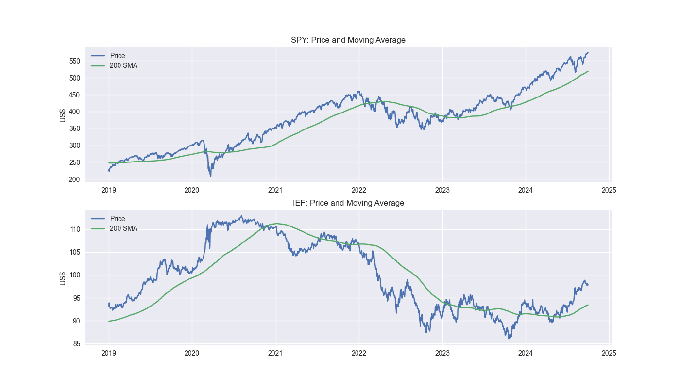
For this test, we’ll be using the SPY and IEF ETFs as benchmarks. The actual strategy will be on the SPY, but we want to include the IEF, which tracks the performance of Treasury notes with maturities of 7-10 years, as most individuals will have some combination of stocks and bonds in their portfolio. Clearly, this will not be an institutional portfolio where one can get paid exorbitant amounts of money to underperform buy-and-hold. But, it should be such a simple benchmark that must should be able to replicate it. The strategy, on the other hand, may not be so. But if turns out to require API calls and connecting to brokerage endpoints, we’ll cover that too – provided the strategy warrants the extra effort.
And since we can’t write a blog post without out at least one graph, we’ll leave you with a plot of the two ETFs and their 200-day moving average. The code follows.
# Built using Python 3.10.19 and a virtual environment

# Load packages
import os
import pandas as pd
import numpy as np
from datetime import datetime, timedelta
import yfinance as yf
import matplotlib.pyplot as plt

plt.style.use('seaborn-v0_8')
plt.rcParams['figure.figsize'] = (14,8)


# Load Data
data = yf.download(['SPY', 'IEF'], start='2000-01-01', end='2024-10-01')
data.head()

# Clean up
df = data.loc["2003-01-01":, 'Adj Close']
df.columns.name = None
tickers = ['ief', 'spy']
df.index.name = 'date'
df.columns = tickers

# Add features
df[['ief_chg', 'spy_chg']] = df[['ief','spy']].apply(lambda x: np.log(x/x.shift(1)))
df[['ief_200sma', 'spy_200sma']] = df[['ief','spy']].rolling(200).mean()

for ticker in tickers:
    df[f"{ticker}_signal"] = np.where(df[ticker] > df[f"{ticker}_200sma"], 1 , 0)
    df[f"{ticker}_strat"] = df[f"{ticker}_chg"]*df[f"{ticker}_signal"].shift(1)


# Plot 200-day SMA
fig, (ax1, ax2) = plt.subplots(2,1)

top = df.loc['2019-01-01':, ['spy', 'spy_200sma']]
bottom = df.loc['2019-01-01':, ['ief', 'ief_200sma']]

ax1.plot(top.index, top.values)
ax1.set_xlabel("")
ax1.set_ylabel("US$")
ax1.legend(['Price', '200 SMA'], loc="upper left")
ax1.set_title("SPY: Price and Moving Average")

ax2.plot(bottom.index, bottom.values)
ax2.set_xlabel("")
ax2.set_ylabel("US$")
ax2.legend(['Price', '200 SMA'], loc="upper left")
ax2.set_title("IEF: Price and Moving Average")

plt.show()