Gaussian gold
Our previous post, used hierarchical clustering to identify market regimes in the gold miners ETF, GDX. This was inspired by a post from PyQuant News that highlighted a longer article from the London Stock Exchange Group (LSEG). In this post, we’ll continue looking at identifying market regimes and using those predictions as signals for a simple trading strategy.
As noted, the LSEG article showed three different machine learning methods to segregate regimes: clustering, Gaussian Mixture Models (GMMs), and Hidden Markov Models (HMMs). In this post, we look at GMMs. We won’t go into the math behind GMMs, but will provide a bit of the intuition. GMMS are models that are a combination of multiple Gaussian or normal distributions. Since most real world data doesn’t conform to a normal distribution, mixing several Gaussians together can (hopefully!) capture the non-normality of the data better. In our case, the algorithm starts with the assumption of two groups (up/down market) and the randomly assigns each daily return to one of those groups. It then computes the probability that that return belongs to the process that generates the up or down cluster and then updates to the values of the distribution parameters (e.g., mean and covariance) to maximize the likelihood of the data. This process allows the model to refine the parameters iteratively to fit the data better.
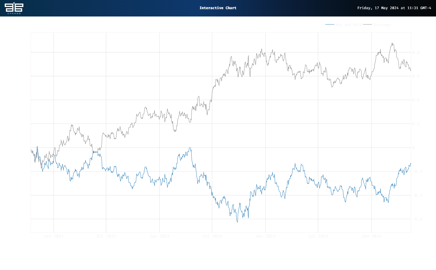
Enough concepts! How does it do? It actually looks too good to be true. While Buy and hold was down a cumulative 14% in the test period, the Strategy was up 65%, almost 80 percentage points of outperformance!
Of course, this is a proof-of-concept backtest, so don’t start using GMMs for all your trade signals. If we shift the start of the trade by one day – a more realistic assumption to counteract the executing the signal right at the close method so many backtests use – we get a much more realistic equity curve, shown below.
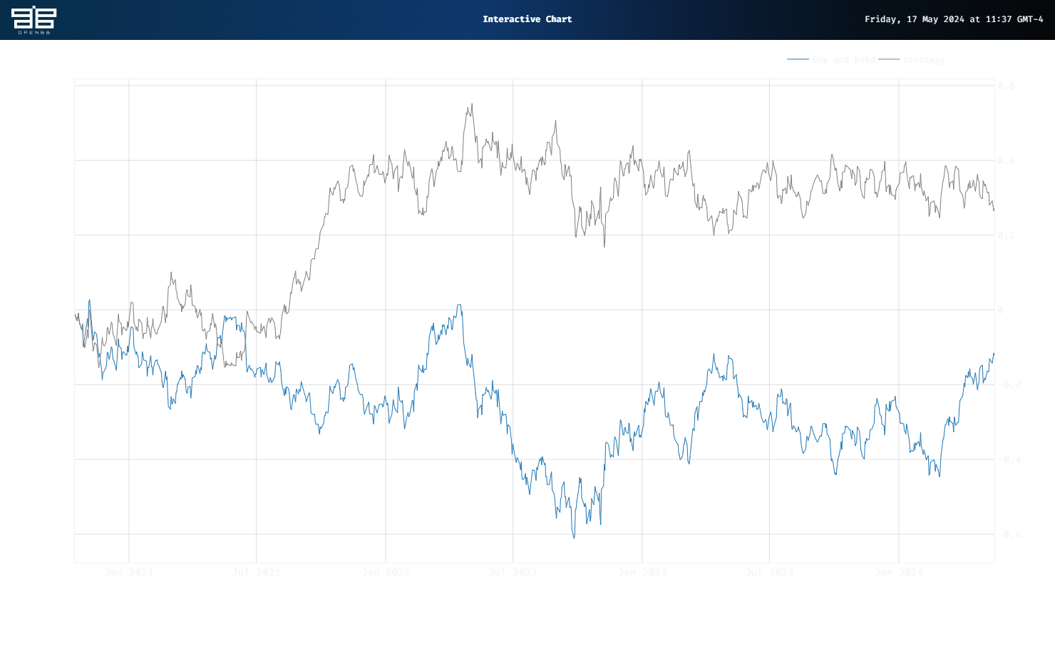
Here, outperformance drops by almost 40 percentage points, but remains positive. Most of the performance occurs in the latter half of 2021, so clearly not a strategy many would want to employ. Nonetheless, the concept remains interesting. We’ll explore HMMs in our next update.
Here’s the code behind the results:
# Built using Python 3.10.19 and a virtual environment

# Install packages
from openbb import obb
import numpy as np
import pandas as pd
from hmmlearn.hmm import GaussianHMM
from sklearn.cluster import AgglomerativeClustering
from sklearn.mixture import GaussianMixture
import math
import warnings
warnings.filterwarnings('ignore')
import yfinance as yf
import matplotlib.pyplot as plt

# Functions
def prepare_data_for_model_input(prices: pd.DataFrame, ma: int, instrument: str) -> pd.DataFrame | np.ndarray:
    """
    Returns a dataframe with prices, moving average, and log returns as well as np.array of log returns
    """
    prices[f'{instrument}_ma'] = prices[instrument].rolling(ma).mean()
    prices[f'{instrument}_log_return'] = np.log(prices[f'{instrument}_ma']/prices[f'{instrument}_ma'].shift(1)).dropna()

    prices.dropna(inplace = True)
    prices_array = np.array([[q] for q in prices[f'{instrument}_log_return'].values])

    return prices, prices_array

class RegimeDetection:

    """
    Object to hold clustering, Gaussian Mixture or Hidden Markov Models
    """
    def get_regimes_hmm(self, input_data, params):
        hmm_model = self.initialise_model(GaussianHMM(), params).fit(input_data)
        return hmm_model

    def get_regimes_clustering(self, params):
        clustering =  self.initialise_model(AgglomerativeClustering(), params)
        return clustering

    def get_regimes_gmm(self, input_data, params):
        gmm = self.initialise_model(GaussianMixture(), params).fit(input_data)
        return gmm

    def initialise_model(self, model, params):
        for parameter, value in params.items():
            setattr(model, parameter, value)
        return model

def feed_forward_training(model: RegimeDetection, params: dict, prices: np.array, split_index: int, retrain_step: int, cluster: bool =False) -> list:
    """
    Returns list of regime states
    """

    # train/test split and initial model training
    init_train_data = prices[:split_index]
    test_data = prices[split_index:]
    if cluster:
        rd_model = model(params)
    else:
        rd_model = model(init_train_data, params)

    # predict the state of the next observation
    states_pred = []
    for i in range(math.ceil(len(test_data))):
        split_index += 1
        if cluster:
            preds = rd_model.fit_predict(prices[:split_index]).tolist()
        else:
            preds = rd_model.predict(prices[:split_index]).tolist()
        states_pred.append(preds[-1])

        # retrain the existing model
        if i % retrain_step == 0:
            if cluster:
                pass
            else:
                rd_model = model(prices[:split_index], params)

    return  states_pred

def get_strategy_df(prices_df: pd.DataFrame, split_idx: int, state_array: list, data_col: str, shift: int = 1, short: bool = False) -> pd.DataFrame:
    """
    Returns dataframe of prices and returns to buy and hold and strategy
    """

    prices_with_states = pd.DataFrame(prices_df[split_idx:][data_col])
    prices_with_states['state'] = state_array
    prices_with_states['ret'] = np.log(prices_df[data_col] / prices_df[data_col].shift(1)).dropna()
    prices_with_states['state'] = prices_with_states['state'].shift(shift)
    prices_with_states.dropna(inplace = True)
    if short:
        prices_with_states['position'] = np.where(prices_with_states['state'] == 1, 1, -1)
    else:
        prices_with_states['position'] = np.where(prices_with_states['state'] == 1,1,0)
    prices_with_states['daily_hmm'] = prices_with_states['position'] * prices_with_states['ret']
    prices_with_states['Buy and hold'] = prices_with_states['ret'].cumsum()
    prices_with_states['Strategy'] = prices_with_states['daily_hmm'].cumsum()

    return prices_with_states

# Get data
symbol = "GDX"
data = obb.equity.price.historical(
    symbol=symbol,
    start_date="1999-01-01",
    provider="yfinance")
prices = pd.DataFrame(data.to_df()['close'])

prices, prices_array = prepare_data_for_model_input(prices, 10, 'close')

# If you want to graph the prices
# line_chart = data.charting.create_line_chart
# line_chart(
#     data=prices,
#     x=prices.index,
#     y="close",
#     title="GDX",
# )

# Create Regime and Backtest
regime_detection = RegimeDetection()
model =  regime_detection.get_regimes_gmm
param_dict = {'gmm': {'n_components':2, 'covariance_type':"full", 'random_state':100, 'max_iter': 100000, 'n_init': 30,'init_params': 'kmeans', 'random_state':100},
              'clustering': {'n_clusters': 2, 'linkage': 'complete',  'affinity': 'manhattan', 'metric': 'manhattan', 'random_state':100},
              'hmm': {'n_components':2, 'covariance_type': 'full', 'random_state':100}
}
params = param_dict['gmm']
split_index = math.ceil(prices.shape[0] *.8)

# Generate regime
states = feed_forward_training(model, params, prices_array, split_index, 20, cluster=False)

# Add to price dataframe
prices['regime'] = np.nan
reg_idx = prices.columns.to_list().index('regime')
prices.iloc[split_index:, reg_idx] = np.array(states)
prices['regime_0'] = np.where(prices.regime == 0, prices.close, np.nan)
prices['regime_1'] = np.where(prices.regime == 1, prices.close, np.nan)

# Get Performance
prices_with_states = get_strategy_df(prices, split_index, states, 'close', short=True)

# Graph result
line_chart = data.charting.create_line_chart
line_chart(
    data=prices_with_states,
    x=prices_with_states.index,
    y=['Buy and hold', 'Strategy']
)

# Get performance from waiting until next day close to execute trade
prices_with_states_1 = get_strategy_df(prices, split_index, states, 'close', shift=2, short=True)


line_chart(
    data=prices_with_states_1,
    x=prices_with_states_1.index,
    y=['Buy and hold', 'Strategy']
)