Risk premia
Our last post discussed using the discounted cash flow model (DCF) as a method to set return expectations that one would ultimately employ in building a satisfactory portfolio. We noted that if one were able to have a reasonably good estimate of the cash flow growth rate of an asset, then it would be relatively straightforward to calculate the required return.
The problem, of course, is figuring out what the cash flow growth rate should be. We examined one workaround, which was to assume that cash flow grows in line with nominal GDP. At first, this seemed a reasonable assumption and we found using GDP performed better than a naive model over short time frames. However, over the long run the two models performed about the same, which implied that there wasn’t much benefit to using a DCF if it performed no better than the naive model, which, in this case, ended up being the historical average return. We discussed using the historical average in an earlier post too.
For this post, we’ll look at the final method for setting return expectations: risk premia. A bedrock assumption of finance (and logic for that matter) is that an asset’s return should be commensurate with its risk. That is, if one asset is riskier than another, then the holder of that asseet should be compensated by a higher return, all else equal. In slightly more technical terms, that required return is the price of risk in the market. Extending this concept, there exists (or at least there is assumed to exist) an overall price of risk in market. Thus, the return on any asset should be a function of the “market’s” price of risk adjsted for that asset’s relationship to the market.
An easy way to see this, using equations, follows. If you don’t like equations just nod your head in agreement.
The return of an asset is based on the Capital Asset Pricing Model (CAPM). We won’t go into the derivation of the model here. But the flow of logic we stated above is elegantly displayed in the equation. Think of this equation as a formalization of those intuitions without worrying too much about the derivation. The equation is:
\[R_{i} = RF + \beta_{i,M}RP_{M}\]
Where:
Ri = return of asset i
RF = risk-free rate
\(\beta_{i,M}\) = beta of asset i with the market
RPM = risk premium of the market, which is the market return less the risk-free rate
The literal translation of the model is an asset’s return is equal to the risk-free rate plus beta times the market risk premium. For now, think of beta as the asset’s relation to the market risk premium.
Thus the model suggests that the return required to compensate an asset’s owner for the risk of that asset should be equal to the overall market price of risk adjusted for that asset’s relation to market risk. If it isn’t, then there’s an arbitrage opportunity: the asset offering a return greater than its price of risk would be bid up and the asset would no longer offer as attractive an investment opportunity.
Let’s parse the model further. First off, it’s a linear model. Beta is the estimated slope coefficient calculated by regressing the return of the asset against the risk premium of the market. This results in a pretty neat insight if we expand beta into its components and rearrange the terms, yielding the following:
\[RP_{i} = \rho_{i,M}\sigma_{i}\frac{RP_{M}}{\sigma_{M}}\]
Where:
RPi = the risk premium of asset i, which is the return of asset i less the risk free rate
\(\rho_{i,M}\) = the correlation between asset i and the market
\(\sigma_{i}\) = the volatility of asset i
\(\sigma_{M}\) = the volatility of the market.
RPM = risk premium of the market, which is the market return less the risk-free rate
What’s elegant about this transformation is that \(\frac{RP_{M}}{\sigma_{M}}\) is essentially the market price of risk, since it is the risk premium of the market per unit of overall market risk. It’s also the market’s Sharpe ratio, a metric we’ve discussed in other posts. So the equation tells you that the risk premium of asset i is it’s correlation with the market times its volatility times the market price of risk. If you know the market price of risk and the other variables, then you can compute the equilibrium risk premium for any asset. Add back the risk-free rate and then you have the expected return.
Beautiful. But is it true? There’s a long history of CAPM bashing, which we won’t rehearse here, but will point out some well-known criticisms.
A particular asset’s relationship to the market may not be linear. This can sometimes be resolved with some sort of transformation, however.
The market’s risk premium or an asset’s sensitivity to the market may not be the only factors driving returns. This has been partially resolved with the Fama-French model and its variations.
Returns don’t increase commensurate with risk. In other words, risk is mispriced or not priced at all. Here is one example.
While these are interesting criticisms, our current project is simply to show how risk premium models work and then test how we can use them to set return expectations. The first hurdle is to find readily available data on global risk premia. Fortunately, Dartmouth Prof. Kenneth French’s data library has a wealth of publicly available data including global market returns. While the data library doesn’t feature an aggregate return for the entire market of risky assets, it does have one for developed and emerging market equities. For now, we’ll use the developed market as a proxy.
First, we’ll pull the data for the S&P 500 and from Prof. French’s library and then graph a scatter plot of the S&P’s monthly returns vs. the market risk premium.
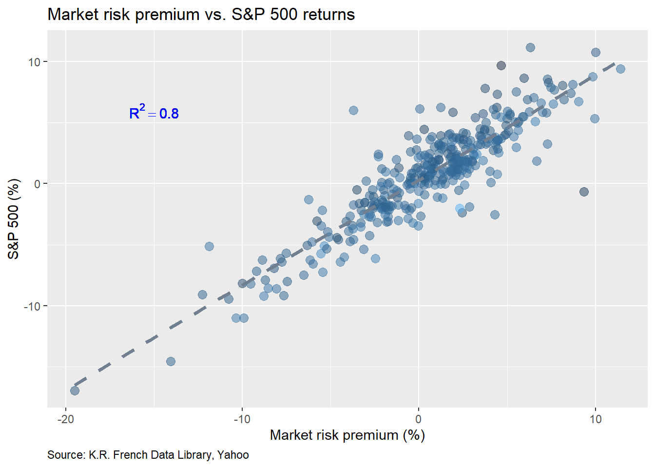
The R2 is quite high at 0.8. But that should be expected given that the S&P 500 is one of the largest indices in the developed markets by market cap, so should have a sizable influence on risk premia. Next we regress the S&P’s return against the market risk premium. The output is below.
| Term | Size effect | Statistic |
|---|---|---|
| Intercept | 0.3 | 3.0 |
| Market risk premium | 0.9 | 37.4 |
The size effect (aka beta) is significant and suggests that for every percentage point move in the market risk premium, the S&P’s return will be almost 9/10ths of a point.
Now we’ll test how well using the historical risk premium predicts the next period’s excess return. Using a rolling 60-month (equivalent to five years) correlation, standard deviation, and average Sharpe ratio we calculate the S&P’s expected return and then compare that with the return for the next month. We substitute p-value for the t-statistic in the output since this might be a bit easier to interpret.
| Term | Size effect | P-value |
|---|---|---|
| Intercept | 1.0 | 0.01 |
| Implied risk premium | -0.7 | 0.24 |
Interestingly, the intercept is significant implying a steady-state excess return of around 1% a month, though such an interpretation might be debatable. Whatever the case, the negative size effect on the market risk premium suggests some mean reversion. However, it is not significant, so we shouldn’t base too much on these results. Indeed, this was just to set up the data. Now we’ll run the same regression annualizing the rolling data to calculate the implied one-year risk premium and then compare that with forward one-year returns.
| Term | Size effect | Statistic |
|---|---|---|
| Intercept | 15.1 | 11.5 |
| Implied risk premium | -1.3 | -7.2 |
We see that based on the t-statistics, the implied risk premium is significant, though the size effect is somewhat counter-intuitive. As we noted above, the negative size effect on the short term model suggested some degree of mean reversion, which made sense as monthly returns are more variable than yearly ones. However, on yearly returns one wouldn’t expect quite so much mean reversion, except that we’re comparing them to the annualized average of monthly returns of the past five years. On this account, the regression results make more sense. As markets experience an upward trend, the expected excess return increases as past average returns are increasing too.1 Yet, just as trees don’t grow to the sky, positive returns don’t last forever. Thus, future returns disappoint. One way to see this is with scatter plot of the S&P 500 vs. the implied risk premium with the points colored by the market price of risk (e.g. the Sharpe ratio). The darker the dot, the higher the Sharpe. Interestingly, the price of risk tends to be highest when the implied risk premium is high relative to returns over the next year.
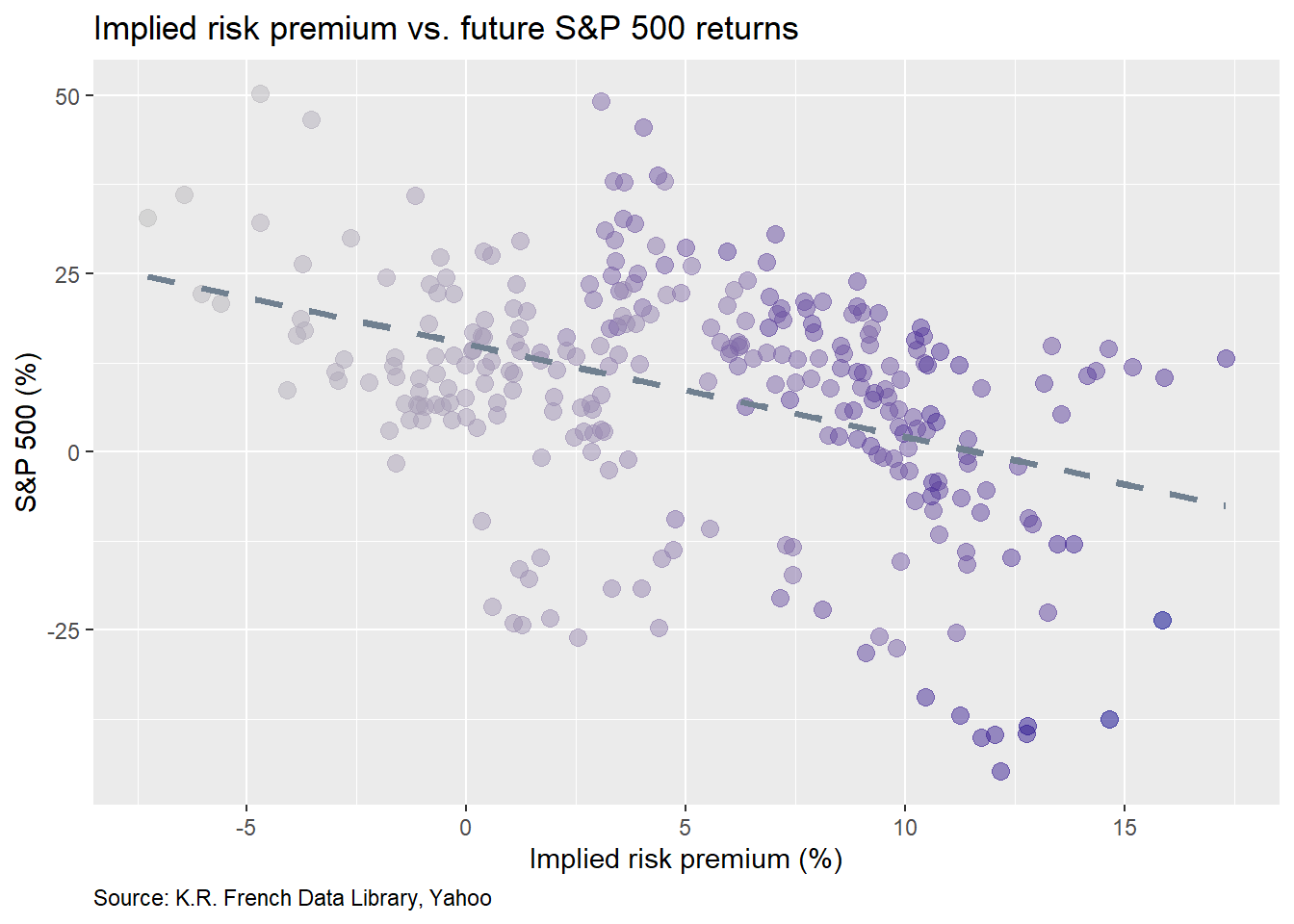
But shouldn’t returns be commensurate with the risk premium? This anomaly is not necessarily a problem with the CAPM, rather our application. The CAPM is not meant to be predictive; rather it is meant to show an equilibrium between the supply and demand of risk. Still, this does present us with a quandary.
If we knew what the market price of risk was going to be in the future along with the other variables, then we should be able to calculate the implied risk premium for our asset of interest. But we don’t know what the future will look like. So the only way to test the predictive power of the principles of the CAPM is to use machine learning principles: train a model, and test it on out-of-sample results. We already did that in one instance with mediocre results. Back to the drawing board.
Perhaps a work around is to bootstrap the regression coefficients from a training set and then test it on out-of-sample data. In this case, we create a training set using 70% of the data, bootstrap the regression coefficients by creating 1000 samples and then use the resulting model to compare predicted results to actuals on out-of-sample data. We show the actual return vs. the fitted return colored by the absolute value of the error in the graph below. The dashed line is the 45o line to show how far off the predicted values are from the actual.
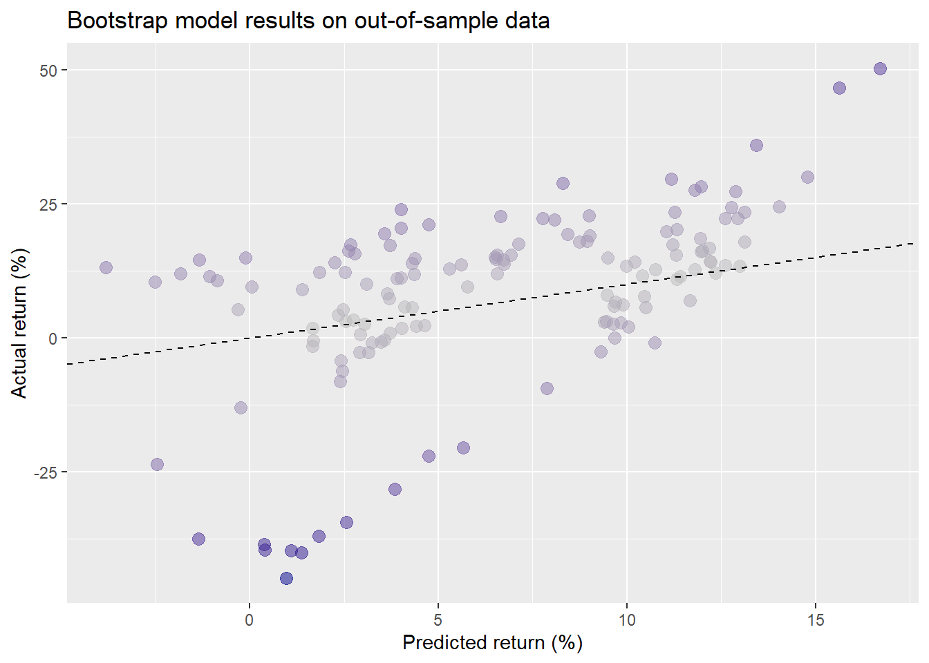
As one can see, the results tend to cluster; do not appear to be randomly distributed; and feature some outliers, all of which suggest that a linear model might not be appropriate. The root mean-squared error of the forecast is around 14 percentage points. The scaled error is about 1.8, meaning that the error is greater than actual average return most of the time.
Even if these stats seem to drive more nails into our model’s coffin, let’s not bury it yet. There are a couple of problems to note. First, linear regression models don’t differentiate between positive and negative returns. Second, we know that financial data is noisy so a linear model will likely have a hard time teasing out the signal.
On the positive vs. negative, most investors are happy if results are better than expected. However, the linear model weights both positive and negative deviations equally and gives even more weight to larger deviations.2
Let’s look at how often the model predicted an up move and down move vs. what happened. In particular, we’re interested in the false positives, or those cases in which the model predicted a positive return and the market was negative.
| Negative | Positive | |
|---|---|---|
| Negative | 3 | 8 |
| Positive | 24 | 102 |
We see that the model predicted a positive return when a negative return actually occurred in 24 of the 27 negative outcomes, equivalent to a false positive rate of 89%. That’s bad. Not quite as bad is that the model predicted a negative return when positive one occurred in eight out of 110 positive outcomes, equivalent to a false negative rate of 7%. So even though the model had a high acccuracy of 77%, its specificity was poor. It’s fine if results are not quite as good as expected, but if they’re negative when expectations are positive, then perhaps the model is best tossed in the dust bin.
On the noisiness of returns, we could bucket the returns to trick the model into thinking there is less volatility. Does it really matter whether the implied risk premium is 5% or 6%? Most folks would say no. Does it matter if it’s 5% vs. 10%? Yes! One way to do this is to transform the returns and risk premia to increments of 5% and then re-run the regression. Unfortunately, the results aren’t much better. (You can verify this by altering the code below.) The reason: future returns still tend to be much different than implied risk premia since the future is, well, unpredictable.
There are other alternatives. One is to build a a time series regression model (auto-regressive moving average, for example) to predict forward risk premia that could then be used to derive a particular asset’s required return. Another is to derive the forward market risk premia by solving for the discount rate that equates future cash flows to the current market price. This is a more complicated version of what we did in Discounted expectations. NYU proferssor and valuation guru Aswath Damodaran regularly calculates such figures and posts the results online.
Both of these approaches could offer promise, but we’d have to test them to be sure, which would require another post. Let’s recap intstead. Besides historical averages, and discounted cash flow models, risk premia is a third way to set return expetations. The intuition is that the supply and demand for risk should be reflected in an equilibrium price. Thus the return of an asset should equal the market price of risk adjusted for that asset’s correlation with the market and it’s specific riskiness. You get what you pay for. However, while the relationship between the market risk premium, the implied risk premium of the asset, and an asset’s return is strong historically, using those relationships to forecast future returns leaves something to be desired; at least for our model using the S&P 500. There may be ways to build a better model, but we’ll have to tackle that in future posts.
The next steps in this series on portfolio construction would be to compare the three capital market expectation models to decide whether one should be preferred over another. We’ve already partially compared the DCF to the historical mean, but haven’t given it our full attention. However, we might spend a little more time on risk premia, given the loose ends mentioned above, before moving on. What’s your opinion? If you want us to investigate risk premia more, or can’t wait to see the back of it, let us know by sending us an email at the address after the code. And now—the moment you’ve been waiting for—here is the code.
## Load packages
suppressPackageStartupMessages({
  library(tidyquant)
  library(tidyverse)
  library(readxl)
  library(httr)
  library(knitr)
  library(kableExtra)
  library(broom)
})

## Load data
sp <- getSymbols("^GSPC", src="yahoo",
                 from="1950-01-01",
                 to="2020-01-01",
                 auto.assign = FALSE) %>%
  Ad(.) %>%
  `colnames<-`("price")

ff_url <- "http://mba.tuck.dartmouth.edu/pages/faculty/ken.french/ftp/Developed_3_Factors_CSV.zip"

GET(ff_url, write_disk(tf1 <- tempfile(fileext = ".zip")))
f_f <- read_csv(unzip(tf1), skip=3) %>%
  rename("date" = X1) %>%
  mutate(date = ymd(parse_date_time(date, "%Y%m"))) %>%
  na.omit()

## Convert S&_ to monthly
sp_mon <- to.monthly(sp, indexAt = "lastof", OHLC = FALSE)
sp_mon_df <- data.frame(date = index(sp_mon), price = as.numeric(sp_mon)) %>%
  filter(date >="1990-07-01")

## Adjust Fama-FRench dates
f_f <- f_f %>%
  filter(date <= "2019-12-31" ) %>%
  mutate(date = sp_mon_df$date) %>%
  mutate_at(vars(-"date"), as.numeric)

## Merge data
sp_df  <-  sp_mon_df %>%
  left_join(f_f, "date") %>%
  mutate(ret = 100*(price/lag(price)-1),
         x_ret = ret - RF) %>%
  rename("Mkt" = "Mkt-RF")

## EDA
rsq <- round(cor(sp_df$ret, sp_df$Mkt, use = "pairwise.complete.obs")^2,2)

sp_df %>%
  ggplot(aes(Mkt,ret)) +
  geom_point(aes(color=SMB), size=3, alpha=0.5) +
  geom_smooth(method = "lm", se=FALSE, color = "slategrey", size = 1.25, linetype="dashed") +
  geom_text(aes(x=-15, y = 6,
                label = paste("R^2 "," == ", rsq, sep="")),
            color = "blue",
            parse = TRUE)+
  labs(x="Market risk premium (%)",
       y="S&P 500 (%)",
       title = "Market risk premium vs. S&P 500 returns",
       caption = "Source: K.R. French Data Library, Yahoo")+
  theme(plot.caption = element_text(hjust=0)) +
  theme(legend.position="")

## Regression
lm(ret ~ Mkt, sp_df) %>%
  broom::tidy()  %>%
  select(term, estimate, statistic) %>%
  mutate_at(vars(-'term'), round, 1) %>%
  mutate(term = ifelse(term == "(Intercept)", "Intercept", "Market risk premium")) %>%
  rename("Term" = term,
         "Size effect" = estimate,
         "Statistic" = statistic) %>%
  knitr::kable(caption = "Regression output Market risk premium vs. S&P 500 excess returns")

# RP look ahead 1 month
one_mon_mod <- sp_df %>%
  mutate(mkt_ret = Mkt+RF,
         corr = runCor(ret, mkt_ret,60),
         ret_sd = runSD(ret,60),
         sharpe = runMean(Mkt,60)/runSD(mkt_ret,60),
         rp_ret = corr*ret_sd*sharpe,
         fut_ret = (lead(price)/price-1)*100) %>%
  lm(fut_ret ~ rp_ret, .)

one_mon_mod %>%
  broom::tidy() %>%
  select(term, estimate, p.value) %>%
  mutate_at(vars(-'term'), round, 2) %>%
  mutate(term = ifelse(term == "(Intercept)", "Intercept", "Implied risk premium")) %>%
  rename("Term" = term,
         "Size effect" = estimate,
         "P-value" = p.value) %>%
  knitr::kable(caption = "Regression output Implied risk premium vs. S&P 500 excess returns")

# RP look head 1 year
one_year_dat <- sp_df %>%
  mutate(mkt_ret = Mkt+RF,
         corr = runCor(ret, mkt_ret,60),
         ret_sd = runSD(ret,60)*sqrt(12),
         sharpe = runMean(Mkt,60)/runSD(mkt_ret,60)*sqrt(12),
         rp_ret = corr*ret_sd*sharpe,
         fut_ret = (lead(price,12)/price-1)*100)

one_year_mod <- lm(fut_ret ~ rp_ret, one_year_dat)

one_year_mod %>%
  broom::tidy() %>%
  select(term, estimate, statistic) %>%
  mutate_at(vars(-'term'), round, 1) %>%
  mutate(term = ifelse(term == "(Intercept)", "Intercept", "Implied risk premium")) %>%
  rename("Term" = term,
         "Size effect" = estimate,
         "Statistic" = statistic) %>%
  knitr::kable(caption = "Regression output Implied risk premium vs. S&P 500 excess returns")

rsq_yr <- round(summary(one_year_mod)$r.squared,2)

rmse <- one_year_mod %>% augment() %>%
  summarise(rmse = sqrt(mean(.resid^2)),
            rmse_mean = rmse/mean(fut_ret))

## Scatter plot
one_year_dat %>%
  ggplot(aes(rp_ret,fut_ret)) +
  geom_point(aes(color=sharpe), size=3, alpha=0.5) +
  geom_smooth(method = "lm", se=FALSE, color = "slategrey", size = 1.25, linetype="dashed") +
  labs(x="Implied risk premium (%)",
       y="S&P 500 (%)",
       title = "Implied risk premium vs. future S&P 500 returns",
       caption = "Source: K.R. French Data Library, Yahoo")+
  scale_color_gradient(low = "grey", high = "darkblue")+
  scale_x_continuous(breaks = c(-5,0, 5, 10 ,15)) +
  theme(plot.caption = element_text(hjust=0),
        legend.position = "")

## Boot strap
library(boot)
set.seed(123)
boot_fun <- function(data,index){
  return(coef(lm(fut_ret ~ rp_ret, data, subset = index)))
}

train <- one_year_dat %>%
  slice(61:205) %>%
  select(rp_ret,fut_ret)

test <- one_year_dat %>%
  slice(206:nrow(one_year_dat)) %>%
  select(rp_ret,fut_ret)

boot_mod <- boot(train, boot_fun, 1000)

boot_pred <- as.numeric(boot_mod$t0[1]) + as.numeric(boot_mod$t0[2])*test$rp_ret

boot_rmse <- sqrt(mean((boot_pred - test$fut_ret)^2, na.rm = TRUE))
rmse_scale <- boot_rmse/mean(test$fut_ret, na.rm=TRUE)

neg_err <- mean(boot_pred >=0 & test$rp_ret < 0)

data.frame(actual = test$fut_ret, y_hat = boot_pred, resid = abs(test$fut_ret - boot_pred)) %>%
  # gather(key, value, - y_hat) %>%
  ggplot(aes(y_hat, actual, color = resid)) +
  geom_point(size = 3, alpha = 0.5) +
  geom_abline(linetype = "dashed") +
  # facet_wrap(~key, labeller = as_labeller(c(actual = "Actual vs. fitted return",
  #                                           resid = "Residuals vs. fitted return"))) +
  scale_color_gradient(low = "grey", high = "darkblue") +
  labs(x = "Predicted return (%)",
       y = "Actual return (%)",
       title = "Bootstrap model results on out-of-sample data") +
  theme(legend.position = "")

tab1 <- data.frame(Predicted = boot_pred, Actual = test$fut_ret) %>%
  na.omit() %>%
  mutate_all(function(x)ifelse(x > 0, "Positive", "Negative")) %>%
  table()

tab1 %>%
  kable(format = 'html',
        caption = "Out-of-sample return occurrences ")  %>%
  add_header_above(c("Predicted" = 1, " \\\ " = 1, "Actual" = 1), line = F) %>%
  column_spec(1, bold = T)

fpr <- round(tab1[2,1]/(tab1[1,1] + tab1[2,1]),2)*100
fnr <- round(tab1[1,2]/(tab1[1,1] + tab1[1,2]),2)*100
Note we’ve substituted excess returns for risk premia. The Sharpe ratio goes up because excess returns increase while volatility stays relatively constant. That means the market price of risk is increasing. Which strikes us as intuitive. As markets climb, one should be compensated to take on more risk since the risk of a decline in values increases. Unfortunately, at some point, you’re not compensated for taking on more risk; in fact, you’re punished. Seems like something’s missing. Or maybe investors aren’t heeding the model!↩
Since the linear model minimizes the squared deviations, large deviations that are double that of small deviations have more than double the impact.↩